The Image Processing One Image tool edit control provides a graphical user interface to the CogIPOneImageTool tool, which implements basic image processing operations such as Gaussian smoothing, high-pass filtering, and image quantization.
Notes:
- The coordinate space tree of the output image is adjusted to preserve the relationship between root space and image features. See the topic Image Processing and Coordinate Spaces for more information.
- The edit control allows you to pick which operators process the input image, in order. The output of the first operator becomes the input image to the second operator, and so on.
- Some image-processing operators support image masking. See the topic Image Processing with Image Masks for more information.
- If the input region for any operator causes the image to become cropped after processing, then any masking parameters or offsets for subsequent operators will be applied using the new coordinates of the cropped output image.
Note:
The following figure shows the One Image Image Processing edit control:
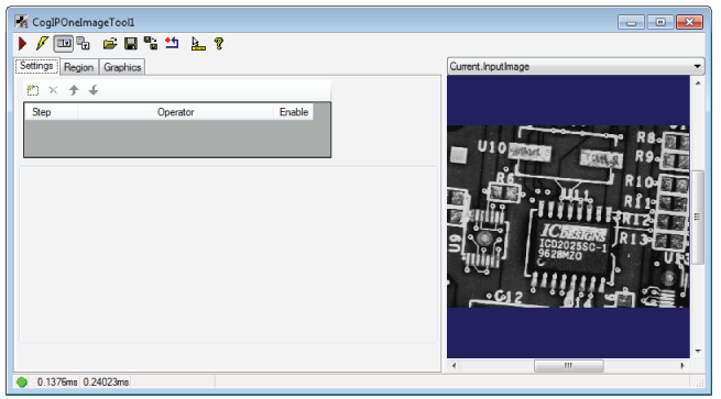
The edit control offers the following features:
- A row of control buttons at the top left provide access to the most common operations.
- A set of function tabs allow you to select the image-processing operations, choose a particular input region, and select display graphics.
- An image display window displays One Image Image Processing tool images and graphics.
To include the edit control in your custom vision application, you must first add it to your Visual Studio .NET development environment. See the topic Adding Edit Controls to Visual Studio for more information.
This topic contains the following sections.

The following table describes the buttons at the top left of the edit control.
| Button | Description | |
 | Run | Perform the selected image-processing operations on the image stored in the Current.InputImage buffer and generate a new LastRun.Output image. |
 | Electric mode | Toggle electric mode, where the tool executes automatically when particular configuration parameters change. In electric mode, a lightning bolt appears next to every electric property. |
 | Local image display | Open or close the local image display window. An Image Processing One Image tool supports the following image buffers:
|
 | Floating image display | Open a floating image window, which supports the same image buffers as the local image display window. |
 | Open | Open a VisionPro persistence (.vpp) file that contains a set of saved properties for this vision tool object type. VisionPro reports an error if you try to open a .vpp file for another object type. For more information about VisionPro persistence features, see the topic Persistence in VisionPro. |
 | Save | Saves the current properties of the underlying tool to a VisionPro persistence file. You have the option to save either the entire tool or the tool without its images or results. |
 | Save As | Saves the current properties of the underlying tool to a new VisionPro persistence file. |
 | Reset | Resets the underlying tool to its default state. |
 | Show ToolTips | Enables or disables the display of tooltips for individual items in this edit control. |
 | Help | Opens this help topic. |
The Image Processing One Image tool edit control allows you to choose the following image processing operations:
| Operator | Description |
Add/Subtract Constant | Add a positive or negative value to the grey value of each pixel in the greyscale image, generating an image that is artificially lighter or darker than the original. Adding a value artificially brightens an image: 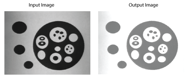 For input images of type CogImage24PlanarColor, values are added to Plane 0 (red), Plane 1 (green), and Plane 2 (blue). The following figure shows an example where the red component has been reduced by a high constant value: 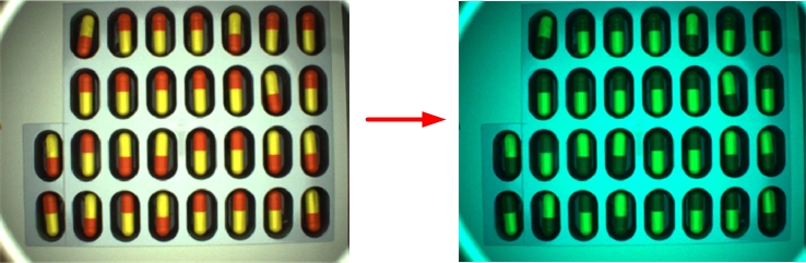 You must also choose whether pixel values that fall below 0 or exceed 255 after the operation are allowed to wrap or be clamped to these limits. For example, in the case of a greyscale image, if you allow the values to wrap then a pixel with a grey value of 200 that has the value 100 added to it has the new value of 45 (200 + 100 - 255). If you choose to clamp the values then the same pixel does not exceed the value 255 after the operation. |
Convolve the input image with a 3x3 kernel of floating-point values. You can use this function, in conjunction with other image processing operators, to implement custom image processing operations, as shown in the following example:  Note that this operator always wraps output values rather than clamping them. | |
Processing the image with a kernel of floating-point values of a size you specify. Use the NxM filter to perform a variety of image processing operations such as edge sharpening, edge detection, and edge softening, as shown in the following example: 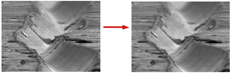 | |
| Equalize | Remap the pixels in the image so that successive acquired images have similar grey values. Use an equalize operation when the lighting in your production environment can vary slightly from one image to the next, or when some aspect of the objects you are inspecting, such as color, are allowed to vary slightly. The equalize operation helps to ensure that irrelevant changes in your production environment do not impact the overall result of the vision application. |
Expand | Enlarge the entire image, or a portion of the entire image, by a magnification factor that you specify. The operation accepts separate parameters for enlarging the image along the x-axis and the y-axis, so you can use the operation to magnify the input image along one direction only. For example, the following figure shows an input image and the image after it has been magnified by a factor of 5:  |
Flip/Rotate | Perform a horizontal flip or a clockwise rotation on all or some portion of the input image. The following figure shows how a portion of an input image has been rotated 180 degrees:  You might need to flip or rotate an image so a vision tool analyzes the correct features each time the application executes, or to use the previously trained font characters of an OCV tool. |
Gauss Sampler | Take a subsample of the input image so that the output image contains only a fraction of the original pixels, and smooth the input image by reducing the amount of contrast caused by frequent changes of light and dark pixels. For example, the following figure shows an image that has undergone a subsampling and smoothing operation:  Use a sampling operation when the vision tools you use work just as effectively on the reduced image and you want to increase the speed of your application. Use a smoothing operation to lessen the effect of liabilities such as texture, signal noise, or fine print in your images. In addition to sampling and smoothing, this operation allows you to include a magnitude shift factor for the output image, with a range of -7 through 7. Using negative values for the shift factor produces darker output images, while using positive values produces lighter output images. |
Perform grey scale morphology on the input image, selectively enhancing or reducing image features based on their size and orientation. See the section Grey-Scale Morphology for background information on this extensive image-processing operation. The following figure shows an image that has undergone a morphological operation:  | |
| Grey Morphology NxM | Perform grey scale morphology on the input image with a kernel of size NxM, selectively enhancing or reducing image features based on their size and orientation. See the section Grey-Scale Morphology for background information on this extensive image-processing operation. |
High Pass Filter | You can perform a Gaussian, Mean or Median smoothing operation and then subtract the resulting image from the input image. The following figure shows an image after a High Pass filter has been applied:  Use a High Pass filter to accentuate fine features in the input image. |
Median 3x3 | Reduce the effect of image noise in the input image by examining the 3x3 matrix of pixels around each original pixel, ranking them by order of grey values, and then taking the fifth, or middle grey value, for the output image. The following figure shows the effect of the median 3x3 operation:  The 3x3 Median operation takes no parameters. Be aware, however, that this operation reduces the size of the input image by 2 rows and 2 columns, or what is effectively a one-pixel strip around the border of the input image. If you use multiple 3x3 Median operations on the same image, the effect of this reduction multiplies. For example, if you use five 3x3 Median operations on an image, the output image will be 10 rows and 10 columns smaller than the original image. |
NxM Median | Reduce the effect of image noise in the input image by examining the matrix of pixels around each original pixel using a kernel of custom size. Larger kernels have a greater effect at reducing image noise but can reduce the quality of features in the image. The NxM Median filter supports a masking kernel of Care and Don't Care pixels, allowing you to specify which elements of the matrix are not considered when generating the new grey value for the output image. Care pixels are enabled as shown in the following figure: |
Missing Pixel | Substitute pixels of unknown value with pixels of a fixed value or pixels whose values are based on the analysis of the surrounding pixels. Pixel values can be unknown based on how they are acquired. For example, range images from a DS1000 series sensor can contain missing pixels. |
Multiply Constant | Multiply the grey value of each pixel in the greyscale image by a constant value. For input images of type CogImage24PlanarColor, the values of Plane 0 (red), Plane 1 (green), and Plane 2 (blue) are multiplied by the multipliers you specify. If you specify a value between 0.0 and 1.0, it has the effect of dividing each pixel by a constant value, as shown in the following figure: 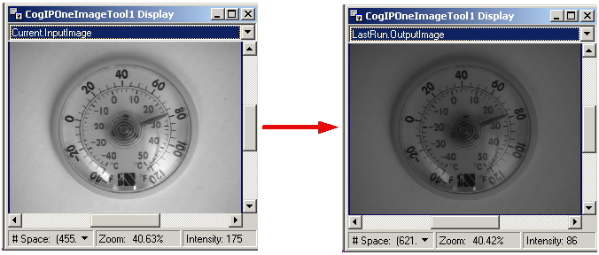 The following figure shows an example where the red component has been multiplied by a high value: 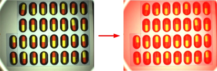 You must also choose whether resulting pixel values that fall below 0 or exceed 255 after the operation are allowed to wrap or be clamped to these limits. For example, if you allow the values to wrap then a pixel with a grey value of 200 that is multiplied by 2 has the new value of 145 (2 * 200 - 255). If you choose to clamp the values then the same pixel does not exceed the value 255 after the operation. |
Pixel Map | Apply a pixel map to the input image. For greyscale input images, each pixel in the input image is replaced by a pixel with the value from the pixel map at the index that is equal to the input image pixel value. For images of type CogImage24PlanarColor, you can specify the individual pixel maps for Plane 0 (red), Plane 1 (green), and Plane 2 (blue). For example, if a greyscale input image pixel has a value of 73, it would be replaced by the value of the 73rd element of the pixel map. The following figure shows the effect of applying an inverted pixel map, where the pixel map contains values from 255 to 0: The following figure shows the effect of applying an inverted Plane 0 (red) pixel map, where the Plane 0 pixel map contains values from 255 to 0: Common applications for a pixel map include constructing mask images and performing customized image equalization. |
Selectively copy input image pixels to the output image or set output image pixel values to a user-defined value, based on which pixels in the input image have been classified as Care or Don't Care pixel values. In many applications the operator uses an image mask to define which pixels you want to pass/set between the input image and the output image. | |
Quantize | Reduce the number of discrete grey values in the input image. Performing a quantize operation can help separate individual features that have similar grey values, or reduce desired features to a single grey value, which can make them easier to analyze with other vision tools. The following figure shows the effect of the quantize operation:  When you select the quantize operation you must choose the number of discrete grey values the output image will contain. |
Sample Convolve | Perform simultaneous separable convolution and sampling. A common use of this is downsampling with Gaussian smoothing. The following figure shows an image that has undergone a smoothing operation: 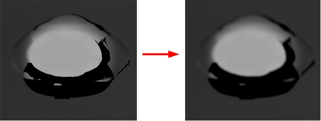 |
Subsampler | Generate an output image where the input image has been reduced in resolution and size. Subsampling can allow other vision tools to operate faster on the reduced image, although reducing the image size can result in less accuracy. The Subsampler operation provides two types of algorithms for generating the output image. The first algorithm divides the input image into blocks of pixels and copies the pixel at the center of the block into the output image. If the block contains an even number of rows or columns, the operation copies the upper-left pixel closest to the center of the block. The following figure demonstrates subsampling with a 3x3 block:  The second algorithm the Subsampler operation offers is spatial averaging, which divides the input image into blocks of pixels, determines the average grey value of the pixels in each block, and places that average into the output image. The following figure demonstrates spatial averaging with a 2x2 block:  Between the two algorithms, the subsampling operation executes faster, but the spatial averaging algorithm offers a higher degree of accuracy. Note: If you specify an even number for the subsampling rate and you do not use spatial averaging, the tool selects the pixel above and to the left of the center of the sampling area. This introduces a one-half pixel shift in the locations of features in the sampled image. The tool automatically adjusts the output image coordinate space tree by shifting the coordinate space by one-half pixel. Because spatial averaging averages pixel values evenly across the sampling area regardless of its size, no such adjustment is performed when spatial averaging is enabled. |
| No Operations | The tool can also be configured to use no image processing operations at all. In this case it simply applies the input region to the input image to produce an output image. This can be useful if you want to affine transform a region of pixels, or want to create a rectangular image this is a copy of some portion of the original input image. |
The following table summarizes the input image types the Image Processing One Image tool supports. The type of the output image will be the same as that of the input image.
| Operation | Method | CogImage8Grey | CogImage16Grey | CogImage16Range | CogImage24PlanarColor |
| Add/Subtract Constant | ✔ | ✔ | ✔ | ||
| Convolve3x3 | ✔ | ✔ | |||
| Convolve NxM | ✔ | ✔ | |||
| Equalize | ✔ | ✔ | |||
| Expand | ✔ | ✔ | ✔ | ||
| Flip/Rotate | ✔ | ✔ | ✔ | ||
| Gauss Sampler | ✔ | ✔ | ✔ | ||
| Grey Morphology | ✔ | ||||
| NxM Grey Morphology | ✔ | ||||
| High Pass Filter | |||||
| Gauss | ✔ | ✔ | ✔ | ||
| Mean | ✔ | ✔ | ✔ | ✔ | |
| Median | ✔ | ✔ | ✔ | ✔ | |
| 3x3 Median | ✔ | ||||
| Median NxM | ✔ | ✔ | ✔ | ||
| Missing Pixel | ✔ | ||||
| Multiply Constant | ✔ | ✔ | ✔ | ||
| Pixel Map | ✔ | ✔ | |||
| Pixel Set | ✔ | ✔ | |||
| Quantize | ✔ | ✔ | |||
| Sample Convolve | ✔ | ✔ | |||
| Subsampler | ✔ | ✔ | ✔ |
This section contains the following subsections.
- Add/Subtract Constant
- Convolve3x3
- Convolve NxM
- Equalize
- Expand
- Flip/Rotate
- Gauss Sampler
- Grey Morphology
- NxM Grey Morphology
- High Pass Filter
- 3x3 Median
- Median NxM
- Missing Pixel
- Multiply Constant
- Pixel Map
- Pixel Set
- Quantize
- Sample Convolve
- Subsampler
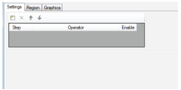
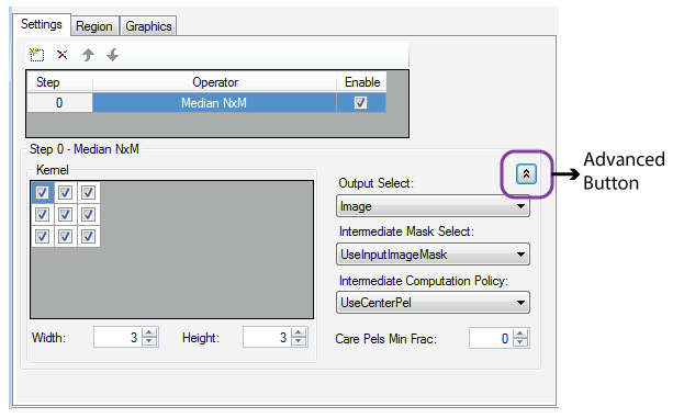
Use the Settings tab to add, configure, and set the order of the image processing operators that the tool applies to the input image. The following figure shows the default Settings tab:
Use the following function buttons to manage the image processing operations:

| Button | Description |
 | Add a new image processing operation. A menu appears with the list of image-processing operations. Highlight the operation you want and a new line appears in the list of image-processing operations at the bottom of the list. You can add more than one operator of the same type. An Image Processing One Image tool with multiple operators exhibits the following behavior:
|
 | Remove the currently highlighted image-processing operation from the list. A verification message appears asking you to confirm deletion. |
 | Move the currently highlighted operation up in the list, and updates the index of the function within the collection. |
 | Move the currently highlighted function down in the list, and updates the index of the function within the collection. |
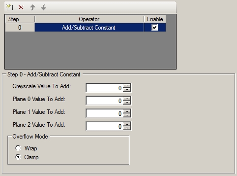
Enter the positive or negative ConstantValue in the Greyscale Value To Add field you want to add to the grey value of each pixel in the greyscale input image. For input images of type CogImage24PlanarColor, enter the positive or negative values for Plane 0 (red), Plane 1 (green), and Plane 2 (blue). You must also choose whether you want to OverflowMode the new values in the output image.
Enter the individual KernelOrigin and to specify the KernelOrigin. (You specify the origin by clicking the option button to the left of the kernel value to use as the origin.)
Specify the KernelHeight and KernelWidth of the kernel, the kernel values, and the BoundaryMode.
The Equalize operation requires no configuration parameters.
Use the Settings tab to enter the magnification factor along the ExpansionX and ExpansionY.
Use the Settings tab to choose how to OperationInPixelSpace the input image.
Use the Settings tab to choose the subsampling factor along the SampleX and SampleY. The larger the subsampling factors you choose, the smaller the output image, while you should choose smoothing factors approximately equal to the size of the features you want to attenuate. You can also choose the smoothing factor along SmoothnessX and SmoothnessY. Enter an optional MagnitudeShift to produce lighter or darker output images.
The Settings tab displays SigmaX and SigmaY values for the standard deviation of grey values of the Gaussian curve along the (x, y) axis.
Click the Advanced button to specify parameters for using image masking:
| Option | Description |
| Output Select | Whether the operator should output just an image, or an image plus a computed image mask. |
| Intermediate Mask Select | Decides whether to use the intermediate image mask, or use the input image mask as the intermediate image mask. |
| Intermediate Computation Policy | How to use the kernel and the input image mask to determine whether to compute a pixel value or copy from the input image. |
| Care Pels Min Frac: | Valid when Intermediate Computation Policy is set to UseCarePelsMinFraction. If the fraction of Care pixels within the kernel of the Input Image Mask are greater than or equal to this setting, use the computed value. Otherwise copy the input pixel value. |
Use the Settings tab to choose the Operation you want the tool to perform. The morphology toolbar
If you choose a Custom structuring element, the Settings tab allows you to configure your own structuring element with the following feature:
Checking a particular MemberMask sets the property for that location in the structuring element to true. While enabled, you can set the GetMemberValue for that location.
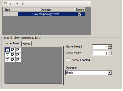
Specify the KernelHeight and KernelWidth of the kernel and use the checkboxes in the Kernel Mask tab to shape the structuring element.
To specify a custom kernel of positive or negative values and further modify how the morphology operator will perform an erosion or dilation, check the Kernel Enabled checkbox and use the Kernel tab to enter the values for the custom structuring element.
When you choose the High Pass Filter operation, the Settings tab shows the following features:
You can choose from the following processing options (CogIPOneImageHighPassFilterProcessingModeConstants):
- Gauss: In Gauss mode, you can specify a smoothing factor along the SmoothnessX and SmoothnessY. The Settings tab also displays the SigmaX and SigmaY values for the standard deviation of grey values of the Gaussian curve along the (x, y) axis.
- Mean: This mode will smooth the input image via a mean filter of user-selectable kernel size. You can specify the KernelHeight and KernelWidth of the kernel.
- Median: This mode will smooth the input image via a median filter of user-selectable kernel size. You can specify the KernelHeight and KernelWidth of the kernel.
| If you are applying a high pass filter to a range image, the Gauss mode is not available. |
The 3x3 Median operation requires no configuration parameters.
Specify the Width and Height of the kernel and optionally specify the Care and Don't Care elements of the processing kernel.
Click the Advanced button to specify parameters for using image masking:
| Option | Description |
| Output Select | Whether the operator should output just an image, or an image plus a computed image mask. |
| Intermediate Mask Select | Decides whether to use the intermediate image mask, or use the input image mask as the intermediate image mask. |
| Intermediate Computation Policy | How to use the kernel and the input image mask to determine whether to compute a pixel value or copy from the input image. |
| Care Pels Min Frac: | Valid when Intermediate Computation Policy is set to UseCarePelsMinFraction. If the fraction of Care pixels within the kernel of the Input Image Mask are greater than or equal to this setting, use the computed value. Otherwise copy the input pixel value. |
Value Computation | Choose the method for determining the value of each missing pixel:
|
Direction | The direction in which missing pixel analysis is to be performed:
|
Global Value Mode | Choose the manner in which the missing is determined when Value Computation is set to Global
|
| Fixed Global Value | The pixel value to use when Global Value Mode is set to Fixed. |
When you choose the Multiply Constant operation, the Settings tab shows the following features:

Enter the positive ConstantValue in the Greyscale Multiplier field by which you want to multiply the value of each pixel in the greyscale input image. For input images of type CogImage24PlanarColor, enter multiplier values for Plane 0 (red), Plane 1 (green), and Plane 2 (blue). You must also choose whether you want to OverflowMode the new values in the output image.
When you choose the Pixel Map operation, the Settings tab shows the following features:
Specify the contents of the pixel SetMap. You can use the grid control to enter individual values in the pixel map, or you can use the Set Linear Map Range controls to set all or part of the map to be a linear mapping. The current pixel map is displayed graphically in the tab. For greyscale input images, set the pixel map by selecting the Greyscale type. For images of type CogImage24PlanarColor, set the individual pixel maps for Plane 0 (red), Plane 1 (green), and Plane 2 (blue).
The Pixel Set operators:
Set the following parameters to use the operator:
Pixel Value: An integer grey value between 0-255.
The grey value you choose depends on your vision application.
Operation: A choice between two options:
- SetCarePels: Set Care pixels in the output image to the value defined by Pixel Value and pass Don't Care pixels directly to the output image unchanged.
- SetDontCarePels: Set Don't Care pixels in output input image to the value defined by Pixel Value and pass Care pixels directly to the output image unchanged.
See the topic Setting Pixels to Defined Values for details on using a Pixel Set operator.

Choose the number of Levels you want the output image to contain.
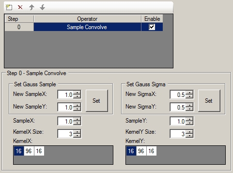
Choose one of the following methods to specify the kernel vectors:
Choose the sample rate in the X direction and the Y direction by entering the values in the New SampleX and New SampleY fields, then click Set.
Once you click Set, the X and Y direction kernels will be calculated and set.
Choose the sigma in the X direction and the Y direction by entering the values in the New SigmaX and New SigmaY fields, then click Set.
Once you click Set, the X and Y direction kernels will be calculated and set.
- You can specify custom X and Y direction kernels by choosing your custom kernel size using the KernelXSize and KernelYSize controls and entering custom kernel values. The sum of the kernel values in each direction may not be greater than 128.
If you want to avoid sampling high frequency details into the result image, perform a blur operation before sampling. You can perform a blur operation with a mathematical convolution with a Gauss function. This convolution is performed in the X and Y dimensions separately.
Note that the exact sample rate and sigma values that the tool will use are displayed in the corresponding tooltips. Because the zero value is invalid for the sample rate or the sigma, if you enter zero for these, it will be substituted by 0.001 automatically.
Choose the level of subsampling along the SampleX and SampleY. You can also choose to use the SpatialAverage algorithm.
Use the Region tab to specify the input region for the tool. The following figure shows the Region tab:
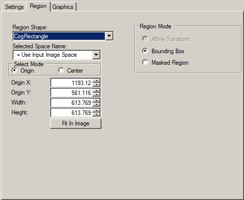
The following table summarizes the features of the Region tab:
| Feature | Description |
Defines how the tool interprets the training region you specify. Choose either of the following options:
| |
Select the shape of the input region. Selecting "None=Use entire image" means that the tool uses the entire input image. An Image Processing One Image tool supports the following input region shapes: The set of region-defining parameters that appear depend on the region shape you use. For more information on using a polygon as an input region, see the topic Using Polygon Input Regions. The tool applies the input region to the input image prior to the first operation only. | |
| Selected Space Name | The coordinate space in which the training region is interpreted. For information, see Coordinate Space Names. |
| Select Mode | Selects the set of parameters that define the rectangle when the available Region Shape is CogRectangle or CogRectangleAffine. If cogRectangleAffine is chosen, the angles of rotation and skew can be specified in degrees or radians, although the underlying tool keeps the measurements in radians. |
Use the Graphics tab to specify the graphics that the tool generates and displays. The following figure shows the Graphics tab:
Choose which of the following graphics appear in the LastRun.InputImage buffer after the tool performs its image-processing operations:
| Option | Description |
| Show Input Images | Determine whether or not the input image is recorded as part of the diagnostic record, and whether the image is copied to the record or saved in the record as a reference. |
| Show Transformed Region Image | Display the affine transformed image, but only if you have specified Affine Transform for the Region Mode and you have supplied a CogRectangleAffine for the input region. |
| Show Region | Display the input region if one was used. |
| Show Intermediate Images | Show the result of each image-processing operation, when multiple operations are configured, as separate images in the display windows. |