In VisionPro, each image has an associated coordinate space tree, and you can define as many Coordinate Spaces as needed for your vision application. Each coordinate space is specified, relative to an existing coordinate space, by a 2D transformation. The coordinate space tree provides VisionPro tools with the information necessary to relate coordinate spaces in your application to pixels in an image or to real-world locations.
Both calibration and fixturing involve calculating a 2D transformation that defines a new coordinate space and then attaching the resulting coordinate space to the coordinate space tree of each run-time image.
See the following sections for more information:
Many vision applications require you to report measurements and locations in meaningful, real-world values. Calibration involves calculating a 2D transformation that maps image coordinates to real-world coordinates, and then attaching this precomputed coordinate space to the coordinate space tree of each run-time image.
Vision tools in the run-time image can report their results in calibrated units.
VisionPro includes two calibration tools, the CogCalibCheckerboardTool and the CogCalibNPointToNPointTool, that perform both of these steps. The two tools take two distinct approaches to the first step of Calibration. The CogCalibCheckerboardTool uses a calibration plate, and it can compute both linear and nonlinear calibrations. The CogCalibNPointToNPointTool requires that you supply information about the locations of a set of points in image and real-world coordinates, and it can only compute linear calibrations.
This section contains the following subsections.
- Checkerboard Calibration Phase
- Grid Point Extraction
- N-Point Calibration Phase
- Run-Time Phase (Both Tools)
- Uncalibrated, Raw Calibrated, and Calibrated Coordinate Spaces
- CogCalibCheckerBoard Tool
- CogCalibNPointToNPoint Tool
- CogCalibNPointToNPoint Tool Summary
- CogCalibNPointToNPoint Programming Model
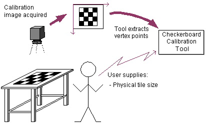
To use the CogCalibCheckerboardTool, you must acquire an image of a calibration plate and provide the spacing of the grid points on the calibration plate in real-world physical units. Your application must call the Calibrate method to perform the calibration. The tool locates the grid point in the plate and computes the best-fit 2D transformation between the real-world coordinates and image coordinates, storing the data for later use. If you need to recalibrate, you must explicitly call the Calibrate method again to obtain a new transformation.
Note: The Checkerboard Calibration tool supports both checkerboard and grid-of-dots calibration plates. Cognex recommends the use of checkerboard calibration plates with the CogCalibCheckerboardTool. Support for grid-of-dots plates is provided for compatibility purposes.
The following figure provides an overview of the calibration phase of the CogCalibCheckerboardTool:
A critical aspect of the calibration phase is the extraction of grid point locations from the image of the calibration plate. The CogCalibCheckerboardTool supports two different types of calibration plates, checkerboard and grid-of-dots plates.
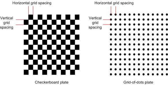
To use a checkerboard plate, where the calibration grid points are the corners of the tiles, you specify the grid point spacing as the tile size. For a grid-of-dots plate, where the calibration vertices are the centers of the dots, you specify the vertex spacing as the dot pitch.
If you are using a checkerboard plate, the tool also lets you specify whether to use standard or exhaustive mode to extract the vertex locations.
Note: Cognex recommends the use of a checkerboard calibration plate with exhaustive feature extraction, as it produces the most accurate calibration. All of the illustrations and descriptions in this topic show the use of a checkerboard plate.
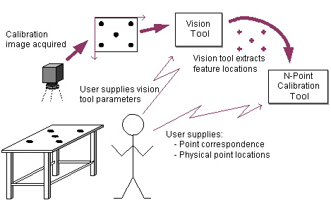
The CogCalibNPointToNPointTool tool requires that you provide a set of points expressed in two different coordinate systems: the real-world physical coordinate system of interest and a coordinate space associated with an image. You specify the location of each point in each coordinate system. As part of this step, you create an image that contains identifiable features with known physical locations. You might, for example, employ a special calibration plate or a circuit board with fiducial markings for which you know or can easily measure distances between features to a high degree of accuracy. The image is usually unlike any other run-time images, except that you acquire it with the same camera and lens that you will use at run-time. You use a search tool to analyze the image of the calibration plate or circuit board and to find the locations of important features. The calibration tool accepts the point coordinates extracted from the calibration image by the search tool. You must explicitly specify the corresponding physical locations (in raw calibrated space) for each point. You then call the tool's Calibrate method. The tool calculates the best-fit, 2D transformation that maps the features in the input image to physical coordinates, storing the data for later use. If you need to recalibrate, you must explicitly call the Calibrate method again to obtain a new transformation.
The following figure provides an overview of the calibration phase of the CogCalibNPointToNPointTool:
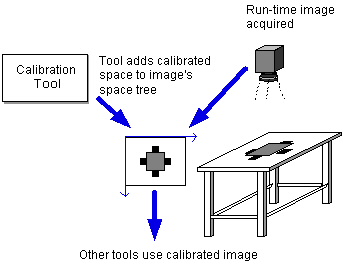
The second step in the calibration process is the same for both calibration tools (when the CogCalibCheckerboardTool tool is used in linear mode): At run-time, the tool attaches the precomputed transformation to a run-time image's coordinate space tree. Once this calibrated space is attached to the image's coordinate space tree, you can obtain the results of other vision tools (such as locations and distances) directly in calibrated real-world coordinates.
The following figure provides an overview of the run-time phase for both calibration tools.
Note: In all cases, the physical and optical set-up must be the same for both calibration-time and run-time operation. The physical and optical set-up includes the lens, camera, and the physical relationship between the camera and scene being acquired. If any of these items is changed, you must re-calibrate the system.
In addition to providing the ability to work directly in calibrated real-world coordinates, both tools let you correct the effects of aspect-ratio distortion caused by non-square camera pixels. The CogCalibCheckerboardTool, when used in nonlinear mode, also lets you correct for the effect of optical and perspective distortion.
Both the Checkerboard and N-Point calibration tools are discussed in more detail later in this topic.
For both calibration tools, the calculation of the best-fit, 2D transformation involves three spaces. These are described in the following table.
| Coordinate Space | Description |
| Uncalibrated | Uncalibrated space is the selected space of the input image before running your calibration tool. It is almost always the pixel-based root ("@") space of an acquired image. |
| Raw calibrated | Raw calibrated space is a calibrated, unadjusted space defined by fitting the physical locations of the raw calibrated points to the uncalibrated points. This space determines the units of the computed calibration transform. It differs from the final calibrated space only in the placement of the origin, which can be rigidly adjusted. |
| Calibrated | The calibrated space is the desired physical coordinate space. It is typically expressed in real-world units, like inches or microns, and aligned with some well-known feature in the physical world. The calibrated space represents the result of the calibration computation. The calibrated space takes into account any rigid adjustment (translation and rotation) you supply. |
Note: The selected space of the calibration image is, by definition, always the uncalibrated space. This is usually the root ("@") space. The selected space of the run-time images must be the same selected space or have the same relationship to the physical world. In practice, this means that you must acquire all calibration and run-time images through the same camera and lens. The camera and lens must also retain their original set-up or calibration time settings. For example, changing the acquisition format (in resolution), moving the camera, or adjusting the focus of the lens will invalidate the computed 2D transformation that maps pixel to real-world coordinates.
You can perform a rigid adjustment of the origin of the final calibrated space by altering:
- The x- and y-translation of the calibrated space origin
- The space in which the translation coordinates are expressed
- The x-axis rotation of the calibrated space
- The space in which the rotation is expressed
- The handedness of the calibrated space
You might, for instance, find it more convenient in your application to place the origin of the calibrated space at the center of an object, rather than at the corner of the image. To achieve this result, you would alter the x- and y-coordinates of the calibrated space. The calculation of the final calibrated space takes into account any rigid adjustments you have made.
The calibration math is equivalent to the following:
UncalibratedFromCalibrated = UncalibratedFromRawCalibrated [ * RawCalibratedFromCalibrated ]
where the portion in brackets represents the rigid adjustment composed of position, rotation, and handedness; and the choice of coordinate space for the position and rotation.
Note: The calibration plates used by the CogCalibCheckerboardTool support the use of fiducial marks that define this rigid adjustment. The fiducial marks indicate the origin, rotation, handedness, and (in the case of grid-of-dots plates), the scale of the rigid transformation. The tool can automatically set these values from the plate.
This section contains the following subsections.
- CogCalibCheckerBoard Tool Summary
- CogCalibCheckerBoard Tool Programming Model
- Nonlinear Mode Differences
As described above, the Checkerboard calibration tool lets you compute a linear 2D transformation between the set of raw calibrated points identified by the grid points of a calibration plate and the locations of those points in the uncalibrated space of an image of the plate. In addition to computing this linear transformation, the tool can also compute a nonlinear transformation that accounts for any optical or perspective distortion introduced by the camera or lens used to acquire the image, and it corrects this distortion by warping the run-time image.
CogCalibCheckerBoard Tool Summary
The following figure provides an overview of both the calibration phase and the run-time phase of the Checkerboard calibration tool:
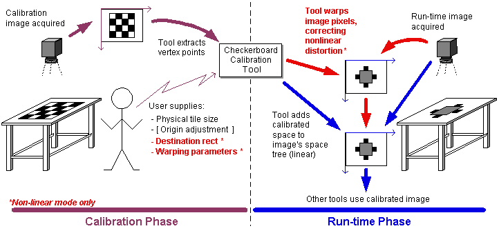
During the Calibration phase, the user supplies an acquired image of the calibration plate, the spacing of the calibration plate grid points in real-world units, and the optional rigid origin adjustment. If you are using the tool in linear mode, the tool automatically extracts the grid point locations from the image of the plate and computes the best-fit 2D linear transformation between the points in raw calibrated space and their locations in the selected space of the calibration image. At run time, the tool adds the linear transformation to the coordinate space tree. Calibration images must be monochrome, however, run-time images can be either monochrome or color.
If you are using the tool in nonlinear mode, then you supply additional parameters related to image warping. In nonlinear mode, the tool automatically extracts the grid point locations from the image of the plate and computes the 2D linear transformation and the non-linear transformation that accounts for any optical or perspective distortion present in the calibration image. At run time, the tool warps the pixels using the nonlinear transformation to produce a corrected image and adds the linear transformation to the coordinate space tree.
See the section Nonlinear Calibration with the Checkerboard Calibration tool for more information on nonlinear calibration and image warping.`
CogCalibCheckerBoard Tool Programming Model
The Checkerboard calibration tool objects are organized in the canonical way for a vision tool that requires a set-up phase. The CogCalibCheckerboard operator holds all the set-up or calibration time parameters; the CogCalibCheckerboardRunParams object supplies the run-time parameters; and the CogCalibCheckerboardTool organizes the input image, run-time parameters, operator, and output image.
The CogCalibCheckerboard operator includes a secondary interface, CogCalibCheckerboard, that defines the parameters used for image warping. For simplicity, you can manipulate this secondary interface directly from a CogCalibCheckerboard object using the OwnedWarpParams property.
The tool contains two sets of N point-coordinate pairs:
- A set that expresses the locations of the N points in uncalibrated space. These locations are the image coordinates at which the tool detected the calibration grid points (tile vertices or dot centers) in the calibration image.
- A set that expresses the locations of the N points in raw calibrated space. These locations are the locations of the grid points in raw calibrated space, based on the location of the origin fiducial mark and the vertex spacing (PhysicalTileSizeX and PhysicalTileSizeX) that you specify.
In addition to supplying the calibration image, you must specify the name of the new calibrated space and the selected space for the output image. This selected space can be either the uncalibrated or calibrated coordinate space.
The tool computes an UncalibratedFromRawCalibrated transform that maps the raw calibrated points onto the uncalibrated points. This transform is returned by the method GetComputedUncalibratedFromRawCalibratedTransform. The computation minimizes the squared error between the corresponding uncalibrated and raw calibrated points. It provides a measure of the mean squared error per point. This computation is performed once at set-up or calibration time and is not recomputed when you run the tool. The computed 2D transform result is stored in the tool's operator, along with a Boolean, Calibrated, indicating that set-up or calibration time results were computed from the current parameters. If any of the parameters change, the operator discards the results and sets the Calibrated Boolean appropriately.
You control which degrees of freedom (for example, rotation and translation) can vary during the calibration computation. You can also perform a rigid adjustment of the final calibrated space by altering the following properties.
- CalibratedOriginX and CalibratedOriginY adjust the x- and y-translation of the calibrated space origin.
- CalibratedOriginSpace adjusts the (x, y) position relative to the uncalibrated (pixel) or raw calibrated (physical) space.
- CalibratedXAxisRotation adjusts the x-axis rotation of the calibrated space.
- CalibratedXAxisRotationSpace adjusts the x-axis rotation relative to the uncalibrated (pixel) or raw calibrated (physical) space.
- SwapCalibratedHandedness adjusts the handedness of the calibrated space.
You can obtain the adjustment transformation by calling GetComputedUncalibratedFromCalibratedTransform. At run-time, the tool attaches this precalculated transform to the coordinate space tree of the input image. It returns a shallow copy of the updated image as output for consumption by other vision tools.
Nonlinear Mode Differences
Most of the information described in the preceding sections applies to both linear and nonlinear mode, but there are some features that are unique to nonlinear mode only.
Unlike the Checkerboard calibration tool, the N-Point calibration tool requires that you extract the features from a calibration image using a vision tool, then provide the feature locations in both raw calibrated space (the real-world locations of the features) and in the calibration image's image space.
The following figure provides an overview of both the calibration phase and the run-time phase of the N-Point calibration tool:
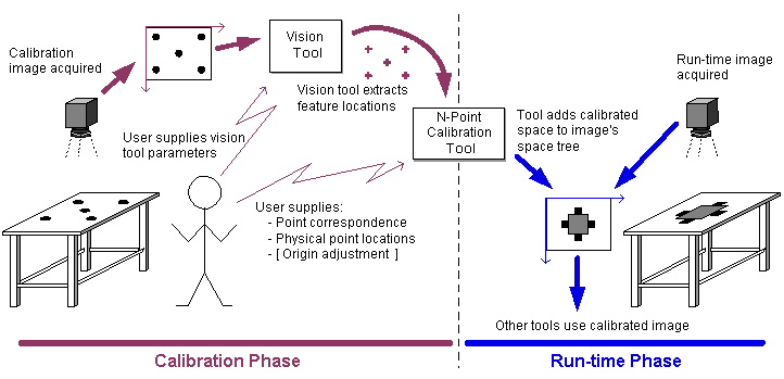
During the Calibration phase, you acquire an image that contains features with known locations in raw calibrated space (real-world coordinates). Using a vision tool such as CogBlobTool or CogPMAlignTool, you locate the image features in the calibration tool's pixel space. You then pass these two sets of coordinates, along with the optional rigid origin adjustment to the tool. The tool computes the best-fit 2D linear transformation between the points in raw calibrated space and the points in the selected space of the calibration image. At run time, the tool adds the linear transformation to the coordinate space tree.
The N-point calibration objects are organized in the canonical way for a vision tool that requires a set-up phase. The CogCalibNPointToNPoint operator holds all the set-up or calibration time parameters; the CogCalibNPointToNPointRunParams object supplies the run-time parameters; and the CogCalibNPointToNPointTool organizes the input image, run-time parameters, operator, and output image.
The tool contains two sets of N point-coordinate pairs:
- A set that expresses the locations of the N points in uncalibrated space. Uncalibrated points are almost always measured in pixels
- A set that expresses the locations of the N points in raw calibrated space. Raw calibrated points are measured in a physical space that is convenient and useful for your vision application
You use other vision tools to search a special calibration image that contains features with known physical coordinates. You supply the locations of found features to the N-point calibration tool as the set of uncalibrated points. You express the set of raw calibrated points in some raw physical coordinate system, using physical values. These points are not measured from an image, and often the physical coordinate system is the desired calibrated space.
In addition, you must specify the name of the new calibrated space and the selected space for the output image. This selected space can be either the uncalibrated or calibrated coordinate space. Note that the SelectedSpaceName of the input image is the uncalibrated space, and points in the uncalibrated point set must be expressed in this coordinate system.
The tool computes an UncalibratedFromRawCalibrated transform that maps the raw calibrated points onto the uncalibrated points. This transform is returned by the N-point calibration method GetComputedUncalibratedFromRawCalibratedTransform. The computation minimizes the squared error between the corresponding uncalibrated and raw calibrated points. It provides a measure of the mean squared error per point. This computation is performed once at set-up or calibration time and is not recomputed when you run the tool. The computed 2D transform result is stored in the tool's operator, along with a Boolean, Calibrated, indicating that set-up or calibration time results were computed from the current parameters. If any of the parameters change, the operator discards the results and sets the Calibrated Boolean appropriately.
You control which degrees of freedom (for example, rotation and translation) can vary during the calibration computation. You can also perform a rigid adjustment of the final calibrated space by altering the following properties.
- CalibratedOriginX and CalibratedOriginY adjust the x- and y-translation of the calibrated space origin.
- CalibratedOriginSpace adjusts the (x, y) position relative to the uncalibrated (pixel) or raw calibrated (physical) space.
- CalibratedXAxisRotation adjusts the x-axis rotation of the calibrated space.
- CalibratedXAxisRotationSpace adjusts the x-axis rotation relative to the uncalibrated (pixel) or raw calibrated (physical) space.
- SwapCalibratedHandedness adjusts the handedness of the calibrated space.
You can obtain the adjustment transformation by calling GetComputedUncalibratedFromCalibratedTransform. At run-time, the tool attaches this precalculated transform to the coordinate space tree of the input image. It returns a shallow copy of the updated image as output for consumption by other vision tools.
When using the N-point calibration tool, keep in mind that a calibration image is not processed in any way by the calibration tool or operator. It is only necessary for visually positioning the origin of the calibrated space in an edit control GUI and by other tools for determining feature locations. Information about an image, such as the locations of feature points, always comes from the analysis performed by another vision tool.
This section contains the following subsections.
Like calibration, fixturing is a two-step process that involves:
- Defining a new coordinate space
- Attaching the space to the coordinate space tree of an input image
You can define any number of coordinate space systems that are specific to your application. Most of these systems have nothing to do with physical units of measurement or correcting optical distortion; they are simply for the convenience of writing your vision application. You frequently perform fixturing prior to making subsequent measurement with a vision tool like CogCaliperTool.
For example, suppose your application ensures that brackets are produced correctly by measuring the distances between two edges on each bracket. The brackets move into camera view on a conveyor belt. You have already calibrated your system and can map image to real-world locations. You would like to use a caliper tool to perform the measurements, however each bracket might have a different location or rotation when you acquire its image. You would like to create a custom coordinate space that moves with each new bracket in each image, so that you can then measure the bracket edges with the caliper.
For each input image, the fixtured coordinate space is recalculated and applied to the image's content. The coordinate axes of the fixtured space remain affixed to the bracket. You use this fixtured space as input to your caliper tool, and can thus measure distances between edges as the bracket's location and rotation change.
All fixturing operations use, at least, the unfixtured and fixtured coordinate spaces. These spaces are described as follows.
- The unfixtured space is the selected space of an input image.
- The fixtured space is a coordinate space that is typically aligned with and conceptually attached to some well known feature(s) in the image. You define the fixtured space to allow you to more conveniently place vision tools or make measurements.
The final fixtured space is represented by a 2D transformation that maps points from the fixtured coordinate space to the unfixtured space.
The CogFixtureTool is very simple. To use it, you must have already obtained a transformation that defines a fixtured space relative to an unfixtured one. The tool performs two tasks at run-time:
- Adds a fixtured coordinate space to the coordinate space tree of an input image
- Creates an output image for consumption by other tools
To complete the first step, you supply the following information to the tool: a nonqualified coordinate space name for the fixtured space; an input image; and a 2D transformation that defines the fixtured space relative to the unfixtured space. You can obtain a 2D transformation from the output of another vision tool, such as PMAlign.
The tool takes the name of the unfixtured space from the InputImage; it is not a property of the tool or run-time parameters.
In the second step, the tool creates a new output image that shares the same pixels and coordinate space tree as the input image. This image is identical to the input image, except that it is a new COM object and it may have a different SelectedSpaceName. The SelectedSpaceName of the output image is either the name of the unfixtured space or the fixtured space, depending upon the value of the tool's SpaceToOutput property. The name is always a fully-qualified space name.
This section contains the following subsections.
- Raw Fixtured Coordinate Space
- N-Point Fixturing Methods
- Reference Fixturing
- Geometric Fixturing
- N-Point Fixturing Objects
- N-Point Fitter
- CogFixtureNPointToNPointTool
Another way that you can create a fixture is by performing N-point fixturing. N-point fixturing lets you define a fixtured space relative to an existing unfixtured space by supplying a set of points expressed in two coordinate spaces. The two spaces are the unfixtured space and a new coordinate space called raw fixtured space. You can also adjust the origin of the final fixtured space.
The raw fixtured coordinate space is a fixtured, unadjusted space defined by fitting the physical locations of the raw fixtured points to the unfixtured points. You can supply the coordinates of a set of N points in this space either using known, real-world measurements or by specifying the points on a reference image.
The raw fixtured space differs slightly from the final fixtured space, because the final fixtured space incorporates an optional origin adjustment. You typically make adjustments (to the translation, scaling, aspect, rotation, or skew) to set up a more convenient location for the final fixtured space. You might, for instance, find it more convenient in your application to place the origin of the fixtured space at the center of an object, rather than at its corner. You alter the appropriate components of the adjustment transform to achieve this result. The fixturing tool first computes the best-fit transformation to map the intermediate or raw fixtured points to the unfixtured points, and then applies the adjustment transform to create the final fixtured space.
The following equation shows how a fixture tool uses the unfixtured and raw fixtured spaces to calculate the final fixtured space.
UnfixturedFromFixtured = UnfixturedFromRawFixtured [ * RawFixturedFromFixtured ]
where the part in brackets represents the optional origin adjustment transformation.
You can choose between two methods of configuring N-point fixturing. These are:
- Reference fixturing
- Geometric fixturing
Both methods use the same math to achieve the fixturing result. The only difference is in how you specify points.
Reference fixturing is the most common method of configuring N-point fixturing. You can use reference fixturing if you do not know the geometric dimensions of your object or the real-world coordinates of points to find within the object before performing fixturing.
In this method, you supply a reference image that shows the physical object to be fixtured. You specify the desired location and orientation of the fixtured coordinate space on the reference image and designate the reference-image coordinates of important object features as raw fixtured points. At run-time, a search tool locates the object features in an input image and feeds the coordinates to an N-point fixturing tool as the set of unfixtured points. These unfixtured points correspond to those specified by the raw fixtured points in the reference-image. The N-point fixturing tool then determines how the features moved between the reference image and the input image, and applies that same movement to the fixtured space defined on the reference image. As object features move from image to image, the fixtured coordinate space axes remain affixed at the same location and orientation on the object.
Suppose, for example, that you want to inspect computer disks. As a first step, you prepare a vision tool, such as PMAlign or Blob, to find the locations of P1, P2, and P3, which are shown in the following figure.
You then acquire a reference image of the disk. The selected space of the reference image is raw fixtured space. Usually, you will use an edit control, such as the N-point edit control to interactively configure the origin and orientation of the final fixtured space on the reference image. The origin adjustment transform is stored, along with the set of raw fixtured points specified by the reference image.
Each time you run the tool, the underlying N-point fixture tool receives a new input image of a disk. The location and orientation of the disk features in the run-time image will typically differ from those in the reference image. The tool calculates the transformation that describes the difference in location and orientation between the (stored) set of N raw fixtured points from the reference image and the (varying) set of N unfixtured points in the input image. It then applies any origin adjustment that you specified. As a result, the final fixtured space has the same relation to the disk features as the fixtured coordinate axes in the reference image: that is, it stays fixed to the disk. You can confirm the correct placement of the final fixtured space by enabling the diagnostic graphic for the fixtured coordinate axes.
When using reference fixturing, you should keep in mind that:
- The reference image is not processed in any way by the tool. The reference image is a convenience for GUI use only in order to position the desired fixtured space.
- You get the coordinates of points from other vision tools. The N-point tools never examine or locate points in images.
- You almost always use the RawFixturedFromFixtured adjustment transform in reference fixturing, because you want to place the final fixtured space in a more convenient location or orientation than the selected space of the reference image.
- You should not need to change the scaling component of the adjustment transform. Usually you have already calibrated your image to determine the scaling factor that correlates image to real-world coordinates. Altering the scaling during fixturing would invalidate the calibrated results.
- Unfixtured and raw fixtured points are often both expressed in root ("@") space. However, this does not imply that the FixturedFromRawFixtured transform is an identity mapping. The points will have different coordinates in the input image and the reference image.
A much less common method of configuring N-point fixturing is geometric fixturing. Geometric fixturing assumes that you have already calculated a calibrated space and that you know the geometry of the object you want to fixture. In this method, you obtain the coordinates of your raw fixtured points either from a schematic (CAD) drawing or from careful measurement of features on the object being fixtured. Geometric fixturing maps the physical, object-local coordinates you supply to the physical locations of the object features in the current input image. It yields a fixture that tracks image content, but also replicates the schematic or model geometry. However, only the rotation and translation degrees of freedom are used by default to calculate the final fixtured space. The math for the geometric fixturing is recalculated for each input image, and you usually do not supply an origin adjustment transform for the final fixtured space.
Because you know the geometry of your object, you can fixture it with a fixturing tool, such as CogFixtureNPointToNPointTool, by matching the known geometric points in the schematic to the found feature locations in your input image. For instance, you may want to create a fixtured space that conforms to the geometry of the computer disk shown in the following illustration.
The origin of the fixtured disk space should be P1, the x-axis extending along the disk's edge toward P2, and the y-axis extending downward. From the schematic drawing, you know the locations of the features in disk space are given by P1 (A, A), P2 (3.5 - A, A), and P3 (3.5 - A, 3 5/8 - A).
You supply these locations to the N-point fixturing tool as the set of raw fixtured points. You run a search tool to find the corresponding locations of P1, P2, and P3 in an input image. The fixturing tool receives these coordinates as the set of unfixtured points. Recall that when you perform geometric fixturing you have already calculated and attached a calibrated space to an input image. The selected space of the input image to the fixturing tool is unfixtured space or, in other words, calibrated space. Unfixtured points therefore have coordinates that are in physical or real-world units. The corresponding set of raw fixtured points has the same units, but assumes a different origin and rotation that helps define the final fixture. Because both the unfixtured and raw fixtured (that is, disk-local) coordinates are already in properly-scaled, physical units, the N-point fixturing tool simply computes the best-fit, rigid transform that matches the constant disk-local coordinates to the found locations of P1, P2, P3 in unfixtured or calibrated coordinates. This is the final fixtured space. Whenever you run the tool, it recalculates the rigid transform to create this disk-local fixture.
Note that you rarely perform geometric fixturing and, instead, will most often do reference fixturing.
VisionPro provides several objects that enable you to perform fixturing. These are the CogNPointToNPoint fitting object and the CogFixtureNPointToNPointTool. The following two sections describe these N-point fixturing objects.
CogNPointToNPoint is a simple N-point fitting object. It is not a tool or an operator, but allows you to programmatically define two sets of N points, group A and group B, and to compute a minimum square error fit between them. It returns a ComputeGroupAFromGroupBTransform that best maps group B points onto the corresponding points of group A. It also returns the root mean squared (RMS) error for the calculation.
The N-point fixturing tool supports N-point-style fixturing operations. The N-point fixturing tool objects are organized in the canonical way for a vision tool that does not have a training phase: The CogFixtureNPointToNPoint operator holds all run-time parameters, the CogFixtureNPointToNPointResult object stores tool results, and the CogFixtureNPointToNPointTool gathers the input image, the operator, and the results.
Like the CogCalibNPointToNPoint tool, this tool contains two sets of N point-coordinate pairs:
- A set that expresses the locations of the N points in unfixtured space
- A set that expresses the locations of the N points in the raw space of the fixture
The corresponding points define the raw coordinate space relative to the unfixtured space. You set up search tools to analyze an input image and supply the unfixtured points to the N-point fixturing tool. You obtain the raw fixtured points using either the reference fixturing or geometric fixturing method.
You must specify the name of the new fixtured space and the selected space for the output image. This selected space can be either the unfixtured or fixtured coordinate space. Note that the SelectedSpaceName of the input image is the unfixtured space, and points in the unfixtured point set must be expressed in this coordinate system. You can also provide an optional adjustment transform (RawFixturedFromFixtured) that lets you create a fixtured space that is more convenient than the one in which the points are originally measured. You might, for instance, want to place the origin of the fixtured space in the center of a located item, rather than at its corner.
As mentioned previously, at run-time, a search tool analyzes an input image and passes a set of unfixtured points to the N-point fixture tool. For each input image, the tool first computes an UnfixturedFromRawFixtured transform that minimizes the squared error between the unfixtured points and the set of previously-specified raw fixtured points. It then applies any optional adjustment transform to calculate the fixtured space. The tool reports the measure of the mean squared error per point, which result you can obtain from the RMSError property. The CogFixtureNPointToNPoint tool then attaches the new fixtured space to the supplied input image and returns a shallow copy of the updated image as output for consumption by other tools.
This section contains the following subsections.
- RMS Error and Degrees of Freedom (DOFs)
- One-Step or Two-Step Calibration and Fixturing
- Running Vision Tools in Fixtured Regions
This section lists some usage guidelines for calibration and fixturing.
Both the N-point calibration and N-point fixturing tools report the root mean squared (RMS) error for the respective calculation of calibrated or fixtured space. The RMS error measures the variation between two sets of N points after calculating the best-fit transformation. It is computed by taking the square root of the mean of the squares of the individual errors, as in the following equation:

Where n is the total number of points, i represents the index of a specific point, and e is the error for a single point. The error is measured in uncalibrated space. It is computed by mapping the raw calibrated position of the point through the calibration transform and then subtracting the mapped result from the found, uncalibrated position of the same point.
You should normally check the RMS error value after computing a 2D transformation that defines calibrated or fixtured space. A large RMS error value may indicate that
- Points may be out of their correct position and therefore measured incorrectly by the tool.
- You do not have the appropriate degrees of freedom (DOFs) enabled.
To reduce the RMS error, you should either modify the points or enable additional degrees of freedom (DOFs). DOFs specify which transformation components the tool can include in its calculation of the best-fit transformation. For example, if the points in one set are scaled, but you have not included scaling in the DOFs, the tool attempts to calculate the best mapping of points that does not vary scaling. If you receive an unacceptable RMS error value as a result, you may be able to reduce it by allowing the tool to consider the scaling degree of freedom in calculations.
In addition, you should be cautious of reporting distances in some fixtured spaces. Although most fixturing operations involve rigid transforms (rotation and translation only) from either calibrated or pixel space, you cannot use a fixture that contains nonidentity scale or skew from a calibrated space to measure distances. In this case, you must first map the fixture points back to calibrated space. You can avoid this problem by only measuring distances and other quantities in calibrated or pixel space; by restricting the degrees of freedom in your fixture space to just allow translation and rotation when computing the best-fit transform between points; or by using only the translation and rotation components of another tool's result transform as input to your fixturing tool.
Vision applications often involve performing both calibration and fixturing. You almost always calibrate an image so that you can report results in real-world values. You may also create a fixtured space that tracks object features so that you can make subsequent measurements of them. If you need only an approximate calibration or if you know the exact dimensions of the part you intend to inspect, you can perform calibration and fixturing in either one or two steps. The following sections describe one- and two-step calibration and fixturing.
In one-step calibration and fixturing, you use the geometric fixturing method to create a fixtured space in physical units. Unfixtured points are typically expressed in a pixel-based space and raw fixtured points are provided in physical units. You supply known geometric measurements or coordinates of your object features, available to you from a schematic (CAD) drawing or physical model. You also enable all degrees of freedom for the fixturing calculation. A new fixtured space is recalculated from the given real-world points each time the tool runs. Because you have enabled all DOFs, the tool considers scaling and skew in the calculation: it treats the known geometric measurements as equivalent to the scaling factor that would be computed by the first step of the calibration process.
One-step calibration and fixturing works for situations where you track and test for the presence or absence of an object feature. For example, you may simply want to fixture a ROI relative to the read-only tab of a 3.5-inch computer disk. You then run a Histogram tool to analyze the brightness levels of the region and determine whether the tab is in the read-only position or not. If the ROI changes in scale, this method keeps the fixtured space always relative to the feature's location.
Note, however, that you should not attempt to measure feature distances or sizes with the one-step calibration and fixturing method, unless you are absolutely certain about the physical position of the features used for fixturing. Suppose, for instance, that you accidentally acquire an image of a 5.25-inch floppy disk. Because you have enabled all DOFs (including scaling, aspect, and skew) and supplied object-local, physical coordinates for a 3.5-inch disk, the tool adjusts the scaling factor of the resulting fixture to allow the 5.25-inch floppy to be 3.5 fixture-units in size. This may still create a fixtured space that tracks a read-only tab, but you cannot validly measure the size of the 5.25-inch floppy. If you did, the floppy would appear to have the same dimensions as the 3.5-inch disk, which obviously does not correspond to the physical size of the floppy. It does not make sense, in this case, to try to measure the physical sizes and distances between object features that were initially used to define the meaning of physical space.
Although you will rarely use one-step calibration and fixturing, you might choose it if you have not already calibrated your input image; you know the physical dimensions of your object; and you only need an approximate calibration. This last criteria may apply if you want to work in (approximate) physical units and:
- You are making only relative measurements (for example, measuring whether the disk hub is centered between the left and right edges of your floppy diskette).
- You are making nongeometric measurements (such as image brightness).
By using two-step calibration and fixturing, you can avoid the drawbacks of the one-step method. In two-step calibration and fixturing, you first perform calibration using the N-point calibration tool to map image to real-world units. You then feed the resulting output image, which has a newly attached calibrated coordinate space, to the N-point fixturing tool and use either geometric or reference fixturing to create a fixtured space. By default, the fixturing tool uses only rotation and translation to calculate the fixtured space. You have already supplied the scaling or skew factors from the calibration tool. You typically choose two-step calibration and fixturing if you need an accurate way to map image features to physical space; have previously calibrated an input image; intend to make measurements in physical space; or want to keep the calibration and fixturing operations separate, performing calibration only once at set-up time.
VisionPro tools always interpret inputs and report results in the selected space of the input image. By default, regions of interest (ROIs) are also interpreted in the selected space of the input image. However, you can set the selected space for a region to a different space than the one in which the tool runs.
Suppose, for instance, that your application requires that you run your vision tool in calibrated space in order to measure results in real-world units, yet also maintain a region of interest affixed to a part within the acquired image. You want a robotic arm to pick up brackets and therefore your application must calculate distances in some calibrated unit, such as microns. You must also track the bracket as it moves in each image, so the robot can determine the proper orientation with which to grasp the bracket.
To accomplish this, you run your vision tool in the coordinate space in which you want your results reported. The selected space name of the input image determines the space in which the tool runs. For the N-point calibration and fixturing tools, you can also specify which space name the tool sets as the selected space name of the output image. To choose the space to output for the N-point calibration or fixturing edit controls in QuickBuild, you use the Space to Output dropdown list on the Settings tab. You then set a different selected space name for the region in which the tool works. For example, in QuickBuild, you choose the selected space name for a region on the tool edit control's Region tab using the Selected Space Name dropdown list.
The following questions can help you determine if you should use a different selected space for your tool and region of interest.
- In what coordinate space do you want your tool's results? To locate the physical coordinates of a part (for example, for robotic picking or placing), you would use calibrated space. If you are measuring relative distances, you can use fixtured space just as well.
- In what region of the input image do you want the tool to run? If you want the tool's region of interest to be fixed to an object that may move from image to image, then set the region's selected space name to the object's fixtured space.
If you chose the same selected space for both questions, you do not need to set different selected spaces. Otherwise, you must specify separate spaces for the tool and region of interest.
This technique saves you the effort of writing code to map tool results from one space to another desired space. In fact, some vision tool results, such as the Blob tool's Perimeter result can be difficult or impossible to map out of the space in which they were originally run.