The 3D Range Image Cross Section Tool allows you to perform measurements on a vertical slice of a range image acquired from a Cognex 3D displacement sensor. There are two main steps: the tool first creates a vertical slice called "profile" from the range image, and then the tool runs a sequence of operators to analyze the profile and make the measurements you desire.

Each of these steps is described briefly below, and in more detail later on.

1. Creating the profile:
   To create a profile you first select a rectangular "slicing" region in the X-Y plane of the range image. This rectangle defines your vertical slice, and is typically long and thin.
   The tool cuts away all range data that falls outside of the region, leaving only the slice. The cut surface of the slice is parallel to the Z-axis of the range image, along the entire boundary of the slicing rectangle.
   The sliced 3D range data is then flattened to 2 dimensions by projecting it onto the plane formed by the centerline of the region as it cut downward along the Z axis. This central plane is called the cutting plane.
   The flattened slice is known as a profile. It represents a sideways view of the average range data at the cutting plane. It is a digital approximation to what you would see if you sliced the range image at the point of the cutting plane and looked in at the data from a viewpoint perpendicular to the cutting plane.
   The profile has its own set of 2D coordinate spaces. These spaces should be thought of as existing in the cutting plane, and are completely different from the 2D coordinate spaces of the range image.
2. Running the operators:
   You can create a sequence of operators that will analyze the profile and make measurements. Each operator can be thought of as a special VisionPro tool that works only on a profile. Each operator has its own parameters, its own results, and its own set of tolerances for those results. The sequence of operators acts like a small toolgroup.
   Operators are of the following types:
   • Operators that extract geometric features (points and line segments) from the profile.
   • Operators that compute new geometric features from existing ones.
   • Operators that make measurements between geometric features.
   You can combine any number of these operators to achieve the measurements that you desire.

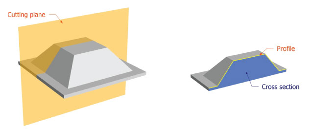
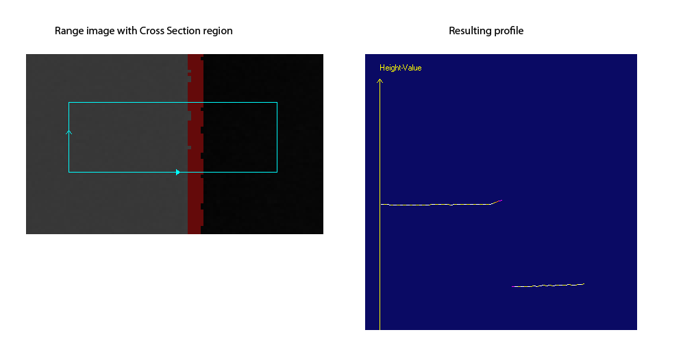
The profile is the contour of the object's cross section that is visible to the sensor.

The following figure demonstrates the profile of an object that the 3D Range Image Cross Section tool returns, using an idealized cutting plane.

The cutting plane is the idealized plane of the cross section and the resulting profile.

The following figure shows the cutting plane on the range image (the plane viewed from the Z-axis), and the resulting profile. As mentioned previously, the infinitely thin cutting plane is actually implemented by taking all of the data in an affine rectangle region and projecting it onto the cutting plane.

The results of the tool are the following:

• The resulting output profile containing the profile data, which is exposed as a property (OutputProfile) of the Cog3DRangeImageCrossSectionRunParams class.
• The results of your measurements, stored in the operators that you use to perform the measurements:
  • The operator's run status
  • The resulting feature or measurement result in the profile coordinate space (defined by the ProfileSelectedSpaceName)
  • The resulting feature in the range image in the 3D range image coordinate space (defined by the SelectedSpaceName3D)
  • The resulting feature in the range image in the 2D range image coordinate space (defined by the SelectedSpaceName)
• The overall status of the operators, which is True if all operators passed and False if at least one operator failed (Status)

Note: The 3D Range Image Cross Section Tool does not have a result class like many other vision tools.

For the theory of range images, acquired from displacement sensors, see the Working with 3D Range Images topic. For information on setting up acquisition with your displacement sensor, see the Getting Started topic. For detailed information on range image acquisition, see the Acquiring Images from a DS900 Series Sensor and Acquiring Images from a DS1000 Series Sensor topics. For advanced range image acquisition details, including coordinate spaces related to range images, see the Range Image Coordinate Spaces and Associated Parameters topic. For hardware-related information (such as mounting and physical product features) and further product details, see the DS900 Quick Reference Guide, DS1000 Quick Reference Guide, and the DS1000 Technical Reference Manual.

The range image slice, based on which the profile is created, is defined by an affine rectangle region lying in the X-Y plane of the range image. The centerline of the region defines the cutting plane. The cutting plane lies parallel to the range image Z-axis.

The following figure illustrates in 3D the region, the cutting plane, and the portion of the inspected object that contributes to the profile generation.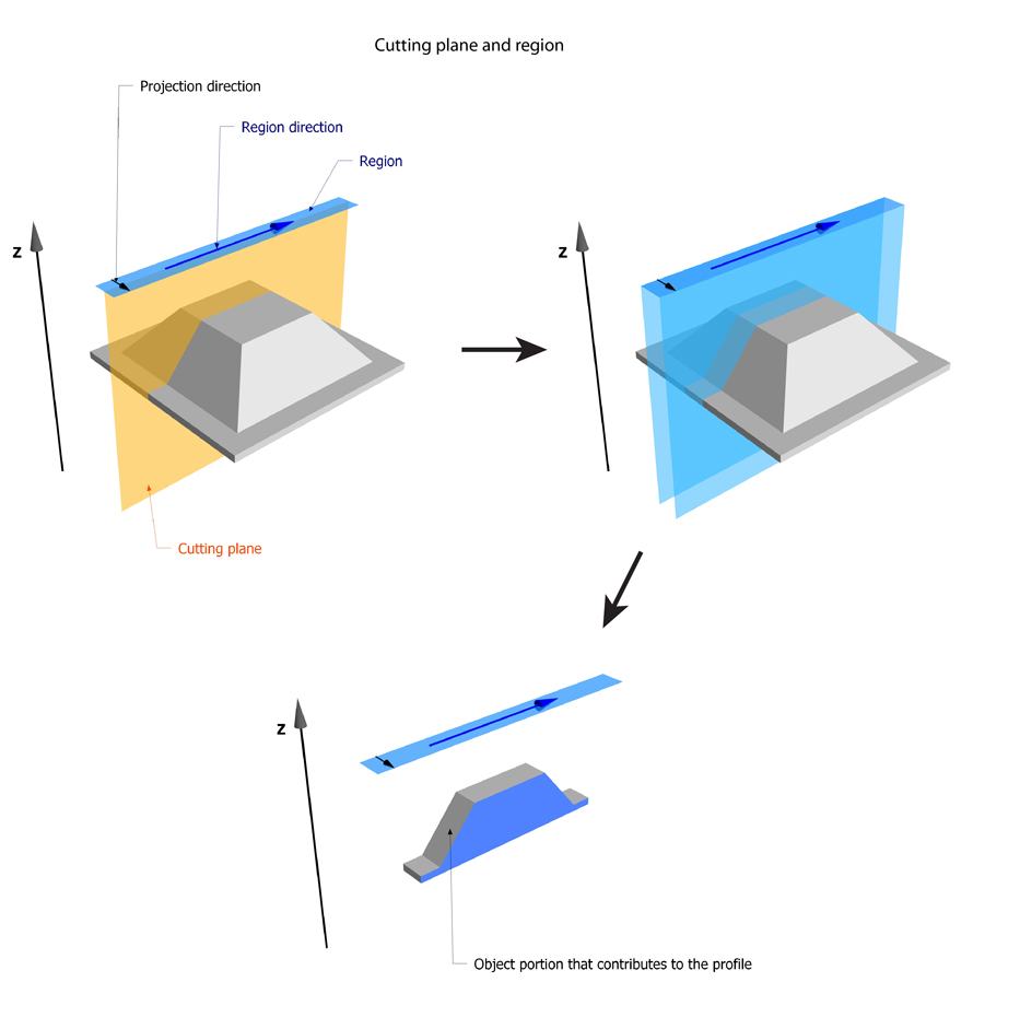

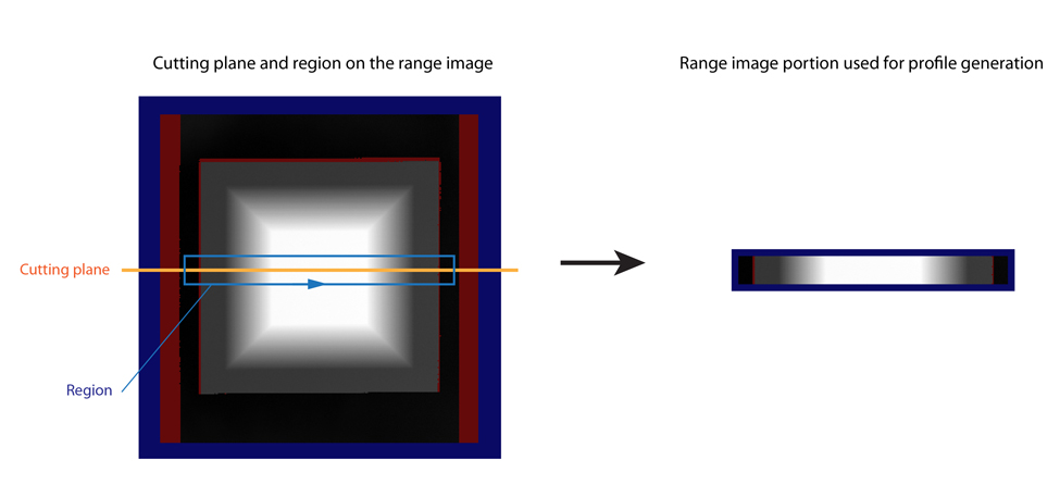
The following figure illustrates on the range image the region, the cutting plane, and the range image portion that contributes to the profile generation. The profile is generated along the region direction using the range image data within the region. The profile is generated in the profile coordinate space, with Region-X and Height-Value axes by default. The profile data at a Region-X value is generated using projection along the projection direction of the region. The projection operation averages all the height information in the projection region along the projection direction, reducing the effects of noise.

The following figure illustrates the projection operation.

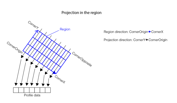
Before averaging, the height information in the region is sampled using bilinear interpolation, similar to the bilinear interpolation described in the Caliper topic. Once sampled, averaging is performed along the projection direction. Only valid (non-missing) pixels contribute to the height value calculation. Missing pixels reduce the weight of a height value.

Specify the region so that the region direction points in the direction in which you want the profile to be created, and the region contains the range image area based on which you want the profile to be created.

You can specify the region in the following ways:

• Supply an affine rectangle using the mouse, defining its location, size and angles of skew and rotation as explained for the Caliper tool in the Specifying the Caliper Input Region topic.
• Define the location, size, and angles of skew and rotation for the projection region numerically using the region parameters.

See the Caliper topic for more information on the theory of affine rectangle regions and their parameters.

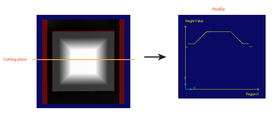
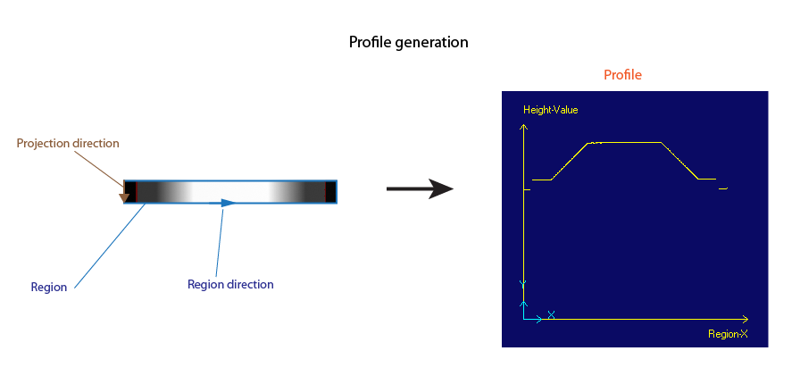
The following figure illustrates profile creation based on the range image portion selected by the region.

To make sure you are viewing the profile of the same portion of each object to be inspected, it is recommended that you fixture the range image region that produces the profile. You can fixture a region in the range image by using the CogFixtureTool. To do this, you first have to find the pattern in the range image that should be the basis of the fixtured range image region coordinate space and then fixture the range image using the pose data of the found pattern. To perform pattern finding in the range image, you will likely have to convert it to a format that your pattern finding tool can take as input.

The raw profile data is expressed in pixels at the root "@" of the ProfileSpaceTree, the Profile2D space is a node in the tree where the profile data is expressed in client units. The profile is drawn in Profile2D.

The drawn profile data is expressed in the profile coordinate space (in mm), which is by default the Profile2D space. The X-axis of the Profile2D space is the Region-X axis, which is aligned with the region direction, and the Y-axis is the Height-Value axis, which is aligned with the Z-axis of the range image coordinate space. The X origin of the Profile2D space is the start of the region crossed by the cutting plane, the Y origin of the Profile2D space is the Z origin of the Sensor3D space associated with the range image.

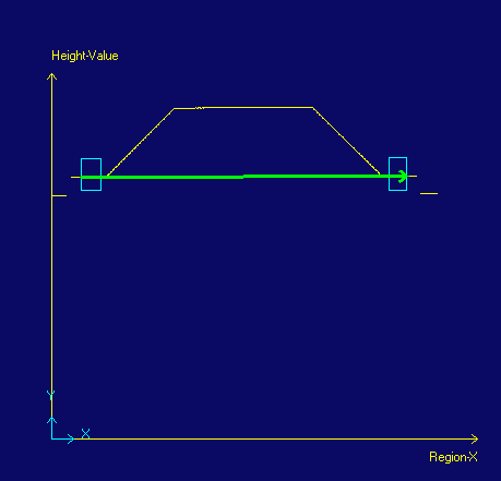
The following figure illustrates the Profile2D space.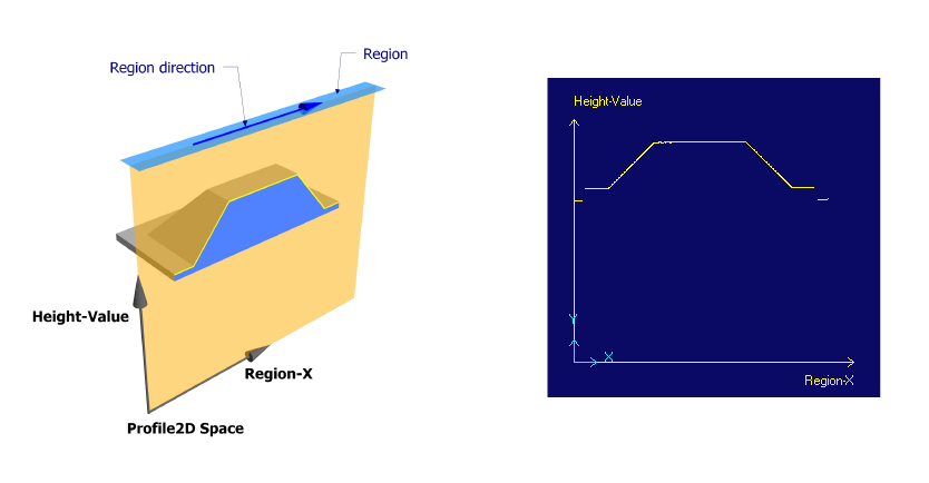

You can change the profile coordinate space to a coordinate space that better suits your application than the default Profile2D space. The profile data will be expressed in the profile coordinate space you specify. You can, for example, fixture your profile coordinate space to a known feature within the profile. You can extract that specific feature from the profile using another Cog3DRangeImageCrossSectionTool and pass its location information to your original tool. That location information can be the origin of your new profile coordinate space. The results of the Cross Section operators are also reported in the space you selected.

The profile owns a CoordinateSpaceTree to which you can add new spaces.

The profile information contains the following items:

• Profile data - the averaged height values along the Region-X axis. This is contained in the Cog3DRangeImageCrossSectionProfileRoot class. The profile data is in pixels.

• Weight data - the ratio between the number of valid (non-missing) pixels along the projection direction (the pixels that contribute to the height value calculation) and the total number of pixels along the projection direction.

  The weight is a value between 0 and 1. 0 means there were no valid pixels at a given Region-X value, 1 means all pixels are valid.

  This is contained in the Cog3DRangeImageCrossSectionProfileRoot class.

• CuttingPlane - the cutting plane.
• ProjectionHeight - the number of pixels in the projection direction.
• ProfileSpaceTree - contains the coordinate space(s) to convert the profile data to the physical units of the range image.

• ProfileSelectedSpaceName - names the coordinate space to use from the profile space tree.

  To map points from the profile data back to the range image and to perform the mapping in the 2D and 3D user-defined spaces:

• CoordinateSpaceTree3D - the 3D coordinate space tree that contains the Sensor3D space.
• PixelFromRootTransform3D - the 3D pixel from root transform that records how the range image pixels within the region were transformed and mangled to become the profile. This transform links the range image coordinate spaces to the profile spaces and defines the bond between the range image pixels and the profile data.
• SelectedSpaceName3D - maps the features found in the profile to the range image.
• CoordinateSpaceTree - the 2D coordinate space tree that references the 2D coordinate space tree of the range image.
• PixelFromRootTransform - the 2D pixel from root transform that is computed from the 3D pixel from root transform.
• SelectedSpaceName - maps the features found in the profile to the range image.

The profile portions with weight = 1 are visualized with alternating bright yellow-white line segments and the portions with 0 < weight < 1 with alternating orange-magenta line segments. Portions with weight = 0 are not visualized.

You work with a profile by using operators in the Cross Section tool. Typically, you will use multiple operators in your application, which are executed in sequence like a toolgroup, to perform the the measurements you desire. Each operator is like a mini-tool that contains its own results and tolerances.

The Cross Section tool's outputs are the profile information, the operator results included in the operators, and the overall status of executing all operators. The overall status is True if all operators passed and False if at least one operator failed.

The following operators are included to work with profiles:

• Extract operators, extracting geometric features from the profile, based on parameters and regions that specify locations in the profile coordinate space.
  • Line segment - extracting a line segment within a region you specify.
  • Point - extracting a point within a region you specify.
  • Corner - extracting a corner within a region you specify.
• Compute operators, computing new geometric features from existing ones. These operators take as input the identity of an operator that produces a geometric feature, which links the consumer of a feature to the operator that produces it.
  • Intersection of two lines
  • Point on a line segment
  • Middle point between two points
  • Line segment between two points
  • Nearest point to line or line segment from a point
• Measure operators, performing measurements between geometric features. These operators take as input the identity of an operator that produces a geometric feature, which links the consumer of a feature to the operator that produces it.
  • Angle between two lines
  • Distance between two points
  • Distance between a point and a line or between a point and a line segment

The following figure shows a case where the angle has been measured between two line segments extracted from two regions. The angle has been found to be 89.88 degrees.

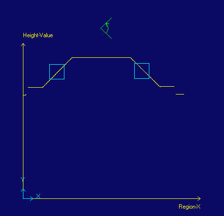
You can also use multiple regions to extract a feature from the profile, which may provide a more accurate result. For example, in the following case, the line representing the rim plane of a frustum is extracted based on two regions.

Your vision applications may get complicated. Sophisticated applications may need to run dozens of operators on a single profile. These applications may also need to run operators in several different profile coordinate spaces on the same profile. To implement these applications, instead of configuring the large number of operators in the single Cross Section tool instance that was used to extract the profile from the range image, you can create multiple Cross Section tools: each tool operates in a single profile coordinate space and each tool can contain an appropriately chosen subset of the desired operators.

To support these use cases:

• The Cross Section tool allows you to create a profile and then pass it to other Cross Section tool instances. Each downstream tool operates on the provided profile without having to (re)define the rectangular region in the range image and without having to extract the profile again. Not having to extract the profile again saves processing time.
• The Cross Section tool allows you to define a new coordinate space, a fixture. The new space can be specified manually or based on an extracted feature.
  • To define the space manually, you will need to specify the name of the space, the translation in X and Y, and the rotation.
  • In most cases though, defining the space will be based on an extracted feature in the profile. By passing the profile from one tool to another, you can create a fixture based on an extracted profile feature.
    Example:
    1. Use tool #1 to create the profile and find a point of interest.
    2. Pass the profile to tool #2 along with the X,Y coordinates of the point.
    3. Use tool #2 to create a new fixtured profile space whose origin occurs at the point of interest.
    4. Use tool #2 to make measurements with respect to the new fixtured space.
• Many Cross Section tools can be used on the profile or the fixture profile to organize the measurements.

To summarize the benefits of profile sharing:

• Not having to extract the profile again, saving processing time
• Not having to specify the region in the range image again
• You can fixture the profile using extracted features from a previous tool
• Not having to specify a large number of operators in one tool
• Not having to fixture the profile again

Note: Even if you choose for your Cross Section tool instance to use an already extracted input profile instead of extracting its own profile, you still have to wire the input image from which the input profile was extracted to your Cross Section tool instance. Each operator provides a specific set of tolerances applicable to the feature or the measurement produced. The tolerances are not enabled by default and you can choose which one to enable. The minimum and maximum tolerance values must be specified with respect to the profile selected space because the values returned are always with respect to the profile selected space.

For example, the following tolerances are available for an extracted line segment:

• RMS - the root mean squared perpendicular error between the line and all of the points in the region
• StartX - X coordinate of starting point
• StartY - Y coordinate of starting point
• EndX - X coordinate of ending point
• EndY - Y coordinate of ending point
• Angle - angle of line

The profile and all of its coordinate spaces represent a completely different view of the range data. The range image is a 3D object and the profile is a vertical slice viewed from the side (out of the range image). Both the range image and the profile have their own coordinate systems.

The region on the range image and regions on the profile are very different things.

Range image related data, which is 3D data:

• The 3D range image itself (described in detail in the Working with 3D Range Images topic).
• The coordinate spaces and transforms associated with the range image (described in the Range Image Coordinate Spaces and Associated Parameters and Working with 3D Range Images topics).
  These include, for example, the Sensor3D space associated with the range image and the PixelFromRootTransform3D transform.
• The affine rectangle region on the range image based on which profile creation is performed, referring to the 3D data in the range image.

Profile information, which is 2D data:

• The 2D profile data and the weight information.
• The profile space tree, which is a 2D space tree that includes the 2D profile coordinate space.
• The affine rectangle regions associated with the operators placed on the 2D profile.