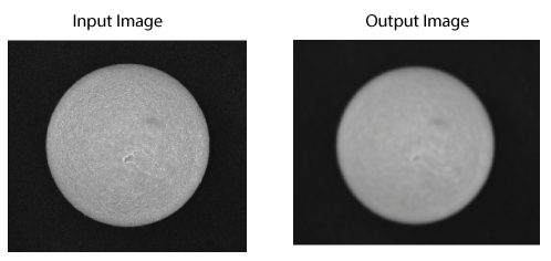
Use a Gaussian Sampling operator on an image to reduce image noise or produce a less-pixelated image, depending on the needs of your vision application:
See the following sections for more information:
This section contains the following subsections.
The Gaussian Sampling operator processes an input image with a Gaussian kernel that approximates a two-dimensional Gaussian distribution. By varying the size of this kernel, the effect of the smoothing can be lessened or increased:

The operator examines the input image for the grey value of each pixel and the pixels surrounding it, takes a fraction of the grey value of each pixel as specified by the kernel, adds these values together, and assigns this new value to the corresponding pixel in the output image:

Note: The values shown may not be actual values that the Gaussian Sampling operator uses in a 3x3 kernel.
Choose a smoothing value which corresponds to the size, in pixels, of the features you want to reduce in detail. The output image is always the same size as the input image.
The operator allows you to subsample the image after smoothing, producing an output image with fewer pixels. Subsampled images can generally be processed more quickly by other vision tools. The image can be sampled at any rate below the smoothing value without loss of information. In general, Cognex recommends you never specify a subsampling rate equal or greater than the smoothing value.
You can specify independent x- and y-axis sampling factors for the Gaussian Sampling tool.
Enhance low-contrast images by specifying a magnitude shift, which performs a bitwise shift of pixel values in the resulting output image. Valid values range from -7 to 7. Negative values will darken the result by dividing the pixel value results by 2 for each bit specified. Similarly, positive values will brighten by multiplying by 2.
A Gaussian curve is a graph of the following function:
where μ is the mean and σ is the standard deviation. The following figure shows a Gaussian curve:
The Gaussian Sampling tool uses an approximation of a two-dimensional Gaussian curve, as shown in the following figure:
You specify the Gaussian kernel size by providing a smoothness value corresponding to the feature size, in pixels, below which you wish to smooth. The relationship between the smoothing value you specify and the size of the resulting Gaussian curve given by the following formula:
where s is the smoothing value and σ is the standard deviation of the resulting curve. The size of the Gaussian kernel itself is then computed using the following formula:

where s is the smoothing value.
Note: You can specify independent values for smoothing in the x- and y-directions, so the kernel might not be square.
| Smoothing | Sigma (s) | Kernel Width |
| 1 | .866 | 4 |
| 2 | 1.414 | 7 |
| 3 | 1.936 | 10 |
| 4 | 2.449 | 13 |
| 5 | 2.958 | 16 |
In general, you should start with a smoothing value of 1 or 2 and increase it until you obtain the desired smoothing.