Analyzing Application Performance with Performance Profiler

The Performance Profiler deploys, runs and monitors tasks in a project to produce a report giving you performance results.

Running the Performance Profiler on Your Application

Run the Profiler to analyze the performance of your application and associated tool blocks in your Task window

1. Click Tools > Performance > Profiler. The Performance Profiler dialog box opens.
2. Select a name (spaces, as well as alphanumeric characters are allowed) and enter it in the Profiler Name field. Make the name descriptive, so you can easily find and reuse the profile later on for other applications.
3. In the Select Tasks field, select all tasks that you want profiled for performance. By default, all tasks are selected.
4. Click Start Deployed Application. The following dialog box will appear.



5. Click Yes. Cognex Designer will display the message Saving... and Deploying... and then shutdown and restart.
6. After Cognex Designer restarts, your product's HMI appears in deployed mode.
7. Run your application, using the HMI. The Performance Profiler will run in the background compiling performance data on your selected tasks. As each Task in your application is profiled, a separate CSV file is created and populated with related performance statistics.
8. Once your selected tasks have executed enough times to gather meaningful data, terminate the application (the HMI). Cognex Designer will shut down and restart with the Tasks_Task.csv_timestamp window displayed, where timestamp is the time the Profiler ran.

Interpreting Performance Profiler Results

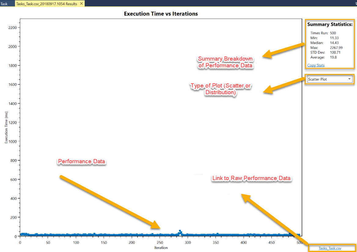
After running the Performance Profiler, a separate Performance Profiler Results window is displayed for each profiled Task with the performance data of each Task diagrammed in a Scatter Plot.

Selecting a Plot Type

You have the option of viewing data as a Scatter Plot or a Distribution Plot. Select whichever you prefer from the Type of Plot drop-down box depicted in the above graphic.

• Scatter Plots are useful for displaying execution times of the task in chronological order .
• Distribution Plots show the distribution of execution times of the task. It is useful for observing how many data points are beyond the norm in a profiling session.

Using Summary Statistics

As depicted in the graphic, the upper-right corner of the Tasks_Task ID Results window lists Summary Statistics, a breakdown of your performance categories using various statistical measurements.

Featured statistics include:

• Times Run - The number of times your task was run.
• Min - Minimum execution time, or the fastest execution time of the selected Task.
• Median - The mathematical median execution time of the selected Task.
• Max - Maximum execution time, or the slowest execution time of the selected Task.
• STD Dev - The amount of variation or dispersion of the selected Task’s execution times.
• Average - The simple mathematical average of all the selected Task’s execution times.

Viewing the Raw Performance Data (CSV) File

To view the complete raw performance data in a CSV file, for viewing in a spreadsheet program such as Microsoft Excel, do the following:

1. Click the highlighted link in the lower-right corner of the Task window.
2. Cognex Designer opens a File Explorer window where you can open a .csv format file with the same name as your Task window.
3. Open the .csv file by double-clicking it. The application you associate with .csv files initializes on your system and opens the .csv file. The .csv file contains a breakdown of performance time for each block defined in your application's Task window along with CPU, memory usage statistics, and Garbage Collection (GC).

Interpreting Raw Performance Data in the CSV File

Use the following table and definitions as a key to the statistics listed in the CSV file. Each row in the CSV file table represents one execution (a single run of the application in the Task window).

Column Descriptor	Definition
ID	The number of executions, starting at zero. For example, a value of zero indicates the first run; a value of 1 indicates the second run, and so on.
Start Time	The time a Task began execution.
End Time	The time a Task ended execution.
Interval	The time difference in milliseconds (ms) between the Start Time of the current run and the Start Time of the previous run. First entry reads NaN (Not a number) as their is no previous run for comparison.
Execution Time	Total time of a particular execution, in milliseconds (ms).
Block Name	Total time that block Block Name took to execute, in milliseconds (ms). This measurement is available for all blocks in your Task window.
GC2	Number of times Second Generation Garbage Collection was called during execution.
GC1	Number of times First Generation Garbage Collection was called during execution.
GC0	Number of times lightweight Garbage Collection was called during execution.
GC Execution Time (M)	Total time in milliseconds that it took all Garbage Collection to complete in manual mode. In other words, Garbage Collection is being explicitly managed by user-written code. This value is only valid when GC Background is disabled. See the topic Scheduling Garbage Collection
GC Execution Time (AD)	Total time in milliseconds that it took all Garbage Collection to complete in dynamic mode. Dynamic mode is obsolete as of release 4.1.0. Garbage Collection is being managed by the settings in Cognex Designer.
GC Execution Time (A#)	Total time in milliseconds that it took all Garbage Collection to complete in automatic mode with background mode disabled. In other words, Garbage Collection is being managed by the settings in Cognex Designer. # is a positive number indicating the set GC Frequency. See the topic Scheduling Garbage Collection   Scheduling Garbage Collection
GC Execution Time (AB#)	Total time in milliseconds that it took all Garbage Collection to complete in automatic mode with background mode enabled. In other words, Garbage Collection is being managed by the setting in Cognex Designer. # is a positive number indicating the GC Frequency.See the topic Scheduling Garbage Collection   Example: GC Execution Time (AB5) indicates that Garbage Collection is called every 5 task executions with GC Background enabled.
ManagedMemoryUsed (MB)	Amount of RAM in megabytes (MB) managed by .NET Cognex Designer process.
TotalMemoryUsed (MB)	Total RAM used by .NET Cognex Designer process.
OnComplete script execution time	Total execution time in milliseconds (ms) of the user script On Complete.
OnError script execution time	Total execution time in milliseconds (ms) of the user's On Error script.

Importing Past Profiler Results

You can open any past Profiler results by clicking Tools > Performance > Import and selecting the raw .csv file of a previous profiler run.

This is particularly helpful when comparing two different profiler runs to verify that performance improvements have made substantial impact.