Count Options and the Confusion Matrix

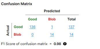
A "count" in the confusion matrix refers to one Actual-Predicted result pair. For example, the confusion matrix below shows the following result counts:

Result Pair	Result Count
Good Actual + Good Predicted	136
Blob Actual + Good Predicted	0
Good Actual + Blob Predicted	1
Blob Actual + Blob Predicted	14

"Blob" here refers to one class of defects, which was defined when labeling Labeling is the process of annotating an image with "ground truth". Depending on the tool that you are using, labeling can take different forms. You label an image set for two reasons: to provide the information needed to train the tool and to allow you to measure and validate the performance of the trained tool against the ground truth. defects for a Standard type Red Analyze tool. The other defect class in this example is "Scratch" and it is not shown in the image because the confusion matrix can only show one defect class at a time.

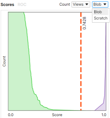
The setting of the Count dropdown menu in the Database Overview determines what results are used for calculating the count in the confusion matrix and ultimately the F1 score. The values shown in the confusion matrix change depending on which option you select.

You can use the Count menu to:

• Base the calculation of the confusion matrix on views or regions.

• Change the shown defect class if you have more than one.

Setting the Count to Be Based on Views or Regions	Setting the Defect Class

Definition of Views and Regions

The terms "view A view of an image is a region of pixels in an image. Tool processing is limited to the pixels within the view. You can manually specify a view, or you can use the results of an upstream tool to generate a view." and "region" correspond to the two types of labeling used for the Red Analyze tool:

• View

  • Corresponds to view-wise labeling and to the Views and Untrained Views options in the Count menu.

  • View-wise labeling involves labeling the entire view as "Good" or "Bad" in the view browser. This method is primarily used with Unsupervised type Red Analyze tools.

• Regions:

  • Corresponds to pixel-wise labeling and the Regions and Untrained Regions options in the Count menu.

  • Pixel-wise labeling involves manually drawing the labels on the image through the Edit Regions menu option. Each drawn label is a region. This method is primarily used with Legacy and Standard type Red Analyze tools.

  • A pixel with no drawn label is considered to be part of the background and labeled as "Good".

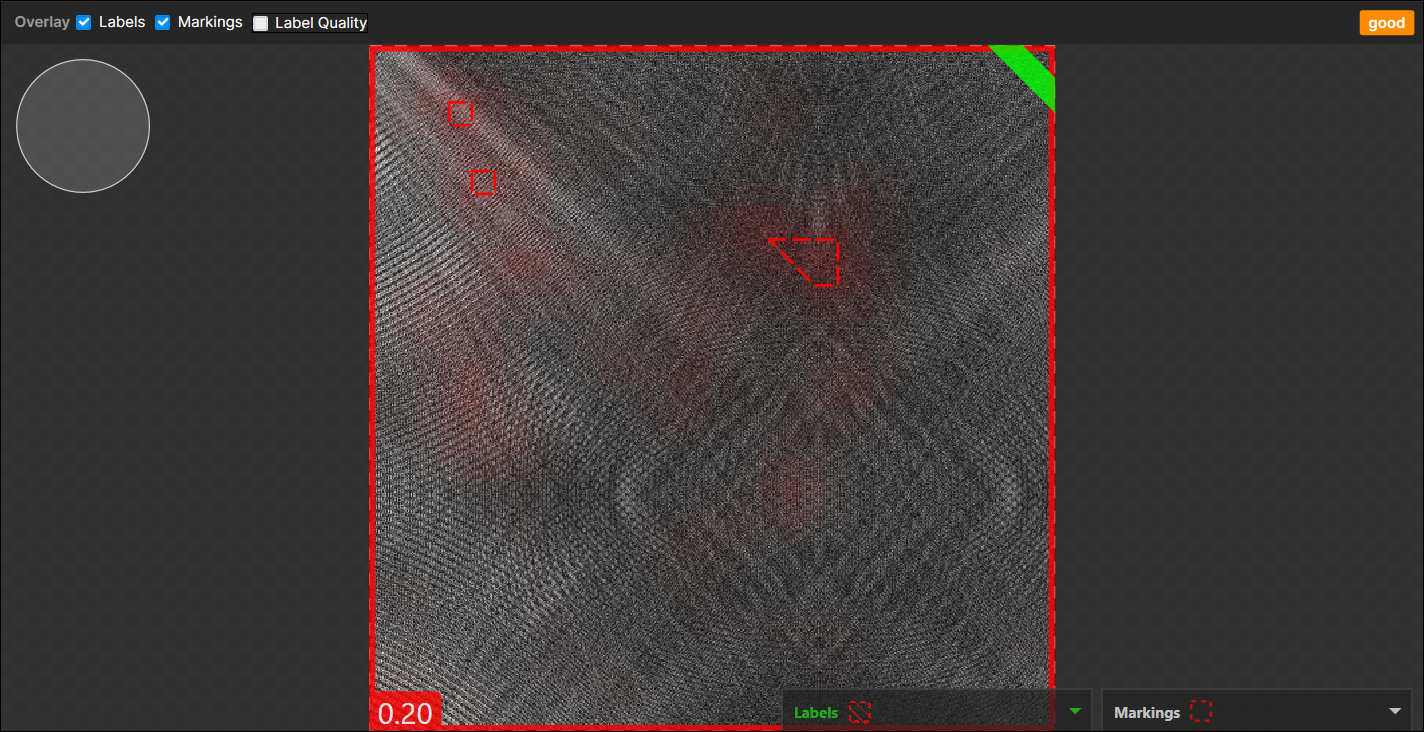
  • The marking Image markings are annotations produced by the VisionPro Deep Learning tools. The markings produced by a tool are the "answers" that the tool obtained when it processed a specific image. You validate the performance of the tool by comparing the markings produced by the tool with the labels that you applied to the same image. As with labels, the specific markings produced depend on the tool. is the prediction of whether a pixel is a defect pixel by checking if the defect probability of the pixel goes over the Threshold. A view that has labeled pixels is automatically labeled as "Bad" on the view level.

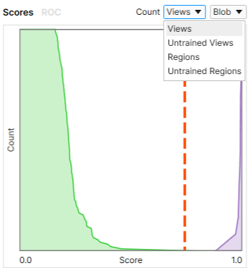
Count Dropdown Options

The Count dropdown menu provides the following options:

• Views: Each view receives a label and a marking.

• Untrained Views: Each view that is not in the training Training is the process that your tool, which is a neural network, is learning about the features (pixels) based on the labels you made. For example, a tool will learn the defect/normal pixels in each image based on the defect/normal labels you drew. The goal of the tool Training is learning enough to give the correct inspection results of whether an unseen image is defective or not. The key to training is to ensure that you include all possible variations within your training set, and that your images are accurately labeled. Training times vary by the application, tool setup and the GPU in the PC being used to train the network. set receives a label and a marking.

• Regions: Each region in a view receives a label and a marking. Regions are split into the defect regions (bad) and the background (good), and labeled and marked accordingly.

• Untrained Regions: Each pixel in a view that does not belong to the training set receives a label and a marking. Regions are split into the defects (bad pixels) and the background (good pixels), and labeled and marked accordingly.

Confusion Matrix Calculation Based On Views

When you set the Count to Views or Untrained Views, the label and the marking is made on each view, not each region. If a view has defect pixels whose score(s) are above the Threshold, then the view is predicted as "Bad". Otherwise, it is predicted as "Good".

To mark a view as "Bad," the defect pixel with the highest defect probability score can be anywhere in a view, not only in the labeled defect region.

In the example below, the defect class "Blob" is selected to represent the "Bad" result. If a view has any defect class other than "Blob", it counts as "Good".

To get the "Actual" counts in the confusion matrix below:

• One view with the label "Blob" counts as "Blob" Actual Blob in the confusion matrix.

• One view with the "Good" label counts as one "Good" Actual.

• One view with a defect class other than "Blob" counts as one "Good" Actual.

To get the "Predicted" results:

• You get one "Good" Predicted result if the highest score from all pixels in a view is below the Threshold.

• You get one "Blob" Predicted result if the highest score from all pixels in a view is above the Threshold.

The prediction is made on each Actual view, not on each region. The prediction is calculated from the Threshold and the representative score of the actual view. The representative score of a view is the highest score of pixels in the view. Each score is the defect probability of each pixel.

Confusion Matrix Calculation Based On Regions

When you set the Count to Regions or Untrained Regions, the labeling and marking are made on each region, not each view. A region is a set of pixels that are marked as defective with respect to the Threshold.

If a view contains multiple marked regions, each region is included in the confusion matrix calculation. This means that a single view can produce multiple counts in the confusion matrix, while a single view only produces a single count in the table if you set the Count to Views or Untrained Views.

In the example below, the defect class "Blob" is selected to represent the "Bad" result again, just as in the previous section. If a view has any defect class other than "Blob", it counts as "Good".

To get the "Actual" counts in the confusion matrix below:

• One view with the "Good" label counts as one "Good" Actual region. The entire view is considered as one background region.

• If a view has regions labeled as "Blob":

  • N number of "Blob" regions count as N number of "Blob" Actuals in the confusion matrix.

  • Additionally, the background region counts as one "Good" Actual.

• If a view has any regions labeled as a defect other than "Blob":

  • M number of regions labeled as other classes count as M number of "Good" Actuals in the confusion matrix.

  • Additionally, the background region counts as one "Good" Actual.

• If a view has both defect regions labeled as "Blob" and defect regions labeled as other defect classes:

  • N number of "Blob" regions count as N number of "Blob" Actuals in the confusion matrix.

  • M number of regions labeled as other classes count as M number of "Good" Actuals in the confusion matrix.

  • Additionally, the background region counts as one "Good" Actual.

• Only Unsupervised type tools: One view with the "Bad" label and with no pixel-wise labeled defect regions counts as one "Bad" Actual region.

To get the "Predicted" counts

• You get one "Good" Predicted result if the highest score from the Actual region is below the Threshold.

• You get one "Blob" Predicted result if the highest score from the Actual region is above the Threshold.

The prediction is made on each Actual region. The prediction is calculated from the Threshold and the representative score of an Actual region. The representative score of the Actual region is the highest score of pixels in the actual region. Each score is the defect probability of each pixel.

Examples of Actual-Predicted Pair Calculation for Regions

In the examples below, we assume that the highest score found from an actual region is above the Threshold.

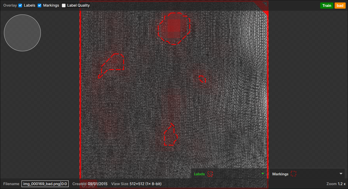
• When N marked regions appear on the backgrounds (the good labeled pixels) and there are no pixel-wised labeled defects and this view itself was labeled as "Good":
  
  → 1 (Actual) Good - (Predicted) Bad pair
  
  (N marked regions are considered as a single marked region)

  Example of 3 marked regions appear on the backgrounds, no pixel-wise labeled defects, "Good" labeled view:
  
  

  

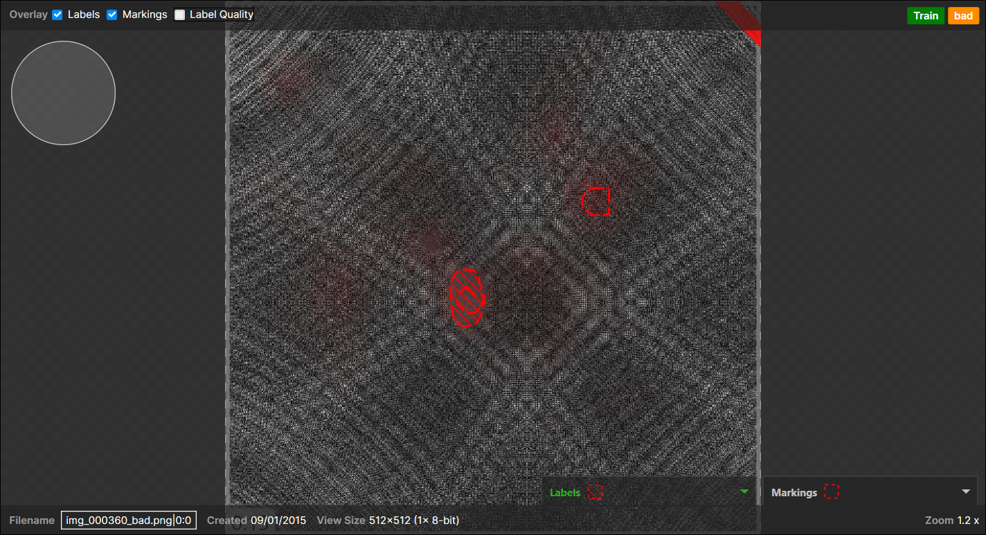
• When N marked regions appear on the background (the good labeled pixels) and there are no pixel-wised labeled defects but this whole view itself was just labeled as "Bad":
  
  → 1 (Actual) Bad - (Predicted) Bad pair
  
  (N marked regions are considered as a single marked region)

  Example of 4 marked regions appear on the backgrounds, no pixel-wise labeled defects, "Bad" labeled view:

  

• When marked regions appear on the pixel-wise labeled defect regions:
  
  The one important thing here to decide the outcome is, of the total, how many marked regions are overlapped with the pixel-wise labeled defect regions:

  • <Case 1>

    1 pixel-wise labeled region,
    
    1 marked region (overlapped with the pixel-wise labeled region),
    
    1 marked region (not overlapped with the pixel-wise labeled region and appear on the background):
    
    →
    
    1 (Actual) Bad - (Predicted) Bad pair (overlapped),
    
    1 (Actual) Good - (Predicted) Bad pair (not overlapped),

    Note: When there are one or more pixel-wise labeled defect regions in a view, all the pixels all of a lump except the labeled regions are considered as "a background," which counts for 1 Actual "Good" region." This expands to most cases but does not apply when there are no pixel-wise labeled regions in the view but the view itself was labeled as "Bad."
    
    

    Example of a marked region appear on the backgrounds, another marked region appear on a pixel-wise labeled region (overlapped), and this view itself is labeled as "Bad" as there are one or more pixel-wise labeled defects:

    

  • <Case 2>

    5 pixel-wise labeled regions,
    
    3 marked regions (each overlapped with each pixel-wise labeled region),
    
    2 marked regions (not overlapped with any pixel-wise labeled region and appear on the background):
    
    →
    
    3 (Actual) Bad - (Predicted) Bad pair (overlapped),
    
    2 (Actual) Bad - (Predicted) Good pair (not overlapped),
    
    1 (Actual) Good - (Predicted) Bad pair
    
    

    Note: The 2 marked regions appeared in the background are considered as a single marked region, which results in 1 "Bad" Predicted. This also expands to the N marked regions case.

  • <Case 3>

    3 pixel-wise labeled regions (A, B, C),
    3 marked regions (2 overlapped with A and 1 with B)
    1 marked region(not overlapped = appear on the background):
    →
    1 (Actual) Bad - (Predicted) Bad pair (2 overlapped with A),
    1 (Actual) Bad - (Predicted) Bad pair (1 overlapped with B),
    1 (Actual) Good - (Predicted) Bad pair (appear on the background),
    1 (Actual) Bad - (Predicted) Good pair (C)